
INTRODUCTION
Many applications in physics are simulated using fractional nonlinear PDEs (FNLPDEs). Even though a lot of academics are willing to study these models, they insist on using different methods to identify answers that are explicit, exact, or approximate. In recent times, a lot of scholars have been interested in solving ODEs, PDEs, and integral equations. Many authors have also concentrated on investigating various methods for solving NLPDEs.
Although fractional derivatives (FDs) are not new to mathematics, their application in research has lagged for a considerable amount of time. The prevalence of non-equivalent formulation of a fractional derivative may be one reason for its disfavor [1]. Furthermore, because FDs are non-local, they cannot be accurately interpreted geometrically [2]. FDs are capable of explaining a wide range of events, such as the nonlinear oscillation of earthquakes [3] as well as the mistake in the fluid-dynamic traffic model resulting from the belief of continuous traffic flow [4]. According to empirical data, fractional order phenomena in DEs and FPDEs for seepage flow in porous media are proposed by [5] and [6], respectively. Mainardi [7] provides an outline of a few uses of FDs in continuous mechanics and statistical mechanics. Numerous authors have studied the analytical findings on the uniqueness and existence of FDE solutions [1, 8]. In recent times, a variety of methods, including Homotopy Analysis and Adomian decomposition, have been employed to solve dynamic systems that comprise FDs, FDEs, FPDEs, and FIDEs [9–13]. Due to their non-local character, fractional operators (FO) are a valuable tool for analyzing phenomena involving the memory effect. We underline that a PDE can be converted from a local to a nonlocal one by substituting a specific FO for the standard derivative with respect to time.
Some of the excellent studies that have been recently covered is the one conducted by Shabir Ahmad et al.[14 – 18] are Dynamical study of a novel 4D hyperchaotic system [14], Dynamical Analysis of Bio-Ethanol Production Model under Generalized Nonlocal Operator in Caputo Sense [15], A hybrid analytical technique for solving nonlinear fractional order PDEs [16], Mathematical Analysis of Biodegradation Model under Nonlocal Operator in Caputo Sense [17] and Analysis of the seventh-order Caputo fractional KdV equation [18].
This essay will solve SFPDEs using the innovative ET method. Boundary value problems are resolved with ET and its variations. The novel process gives better accuracy since different initial approximations are used in all iteration of the solution, in contrast to the recommended approach [17], which puts the result in a finite series form which is simple to calculate. A number of the difficulties are addressed using the general explanation of the suggested remedy. Finding analytical solutions with ICs for FCSNLPDEs is challenging. The current work uses a relatively simple to comprehend and implement approach to produce closed-form analytical solutions for the FCSNLPDEs.
The suggested method offers a fresh approach to broadening the use of fractal techniques to a variety of systems with highly accurate results. This method may show great promise in the near future for creating and using intricate fractal models in a variety of domains, including engineering and physics. The freshly developed method has two distinct features: it is simple to use and offers recommendations for choosing the initial iteration, selecting the first iteration is crucial since it can initiate the method's convergence and enable the calculation of the exact solution in a limited number of steps, if the ICs are exactly zero, we can choose the first iteration all or a subset of the inhomogeneous terms.
Because this method relies entirely on the ET transform and initial conditions, it will be ineffective if the ET is missing for the fractional derivative or if the initial conditions are not present. Also, if the initial iteration is not chosen correctly, we may not reach a convergence to the exact solution.
In this paper, we employ a particular analytical method that utilizes the ET to solve FCSNLPDEs. Examples are given to illustrate this method's efficacy and dependability. This method can be used to solve functional equations that arise from numerical modeling of many processes.
Definition 1: Following are the definitions for the Riemann-Liouville (R-L) operator of order
Properties of Jα,
For Φn ∈ Cμ, n ∈ N, κ, λ ≥ 0 and λ ≥ –1:
Definition 2: As stated by Caputo, the FD of ϕ(B) is:
for m – 1 < κ ≥ m, m ∈ N, B < 0, and Φ ∈To find an FD's correct order, one computes an ordinary derivative first, followed by a fractional integral.
Just like the R-L fractional integral operator, the integer-order integration is a linear process:
[10], explains that FD is believed to possess a Caputo meaning in the current inquiry, which supports the application of the Caputo definition. One of the great advantages of the Caputo fractional derivative is that it allows traditional initial and boundary conditions to be included in the formulation of the problem. In addition, its derivative for a constant is zero, therefore, Caputo fractional derivative was chosen in this paper.
ELZAKI TRANSFORM
In general, the ET is described as:
o is a complex value.PDEs, ODEs, and integral equations in [1–4] and [23–25, 27–32] can all be resolved with ET. Effective application of ET is possible while Sumudu and Laplace transforms fail to handle DEs having variable coefficients [26].
Theorem 1: [2] The partial derivatives are converted by ET in the following ways:
ET of some functions:
In this instance, we offer a few lemmas that enable function ϕ(A) inference from its ET.
Lemma 1: ETof R-L operator of order κ > 0 is
Proof: We establish by
whereLemma 2: ET of Caputo fractional (CF) derivative for
is orThe following is the definition of the Mittag-Leffler functions:
Where Γ is the gamma function and κ,λ are complex parameters with real part are zero.
Lemma 3:
If κ, λ > 0, a ∈ C and
Proof:
Then
THE NOVEL ANALYTICAL METHOED
The primary concept of the suggested plan of study will be made clearer by applying the SFPDE in the following ways,
2
Where
Taking ET of Eqs. (2), to get:
4
Solutions of Eqs. (2), should be performed using the series form that follows:
Using Eqs. (5) and the inverse of ET to Eqs. (4), to get:
6
G1(υ, τ), G2(υ, τ) are the terms found that come from the source terms and the ICs.
This approach is dependent on how we select the initial iterations P0, Q0 that yield the precise solutions in a constrained amount of steps. The solutions P(υ, τ), Q(υ,τ) can be found iteratively using the following relations
7
From Eqs. (7) and (4), we can determine that:
using Eqs. (5) to find the solution.
ILLUSTRATIVE EXAMPLES
Using the process described in this study, we produced the exact solutions for FCSNLPDEs and compared them with the known exact solutions.
Example 1: Consider the FCSNLPDE
with the ICsUsing the ET of Eqs. (8) and ICs, to get:
Inverse ET shows:
The iteration formulas that utilize an initial approximation are as follows:
10
Then we find:
Then, using (5), to get:
If κ = 1, then:
Example 2: Consider the FCSNLPDE
with the IC and BCsUsing similar steps as in example 1, to obtain:
The recurring connections are as follows:
13
From Eqs. (13), we get:
Using Eq. (11) to get:
The subsequent exact solutions can be obtained if κ = 1,
NUMERICAL SIMULATIONS
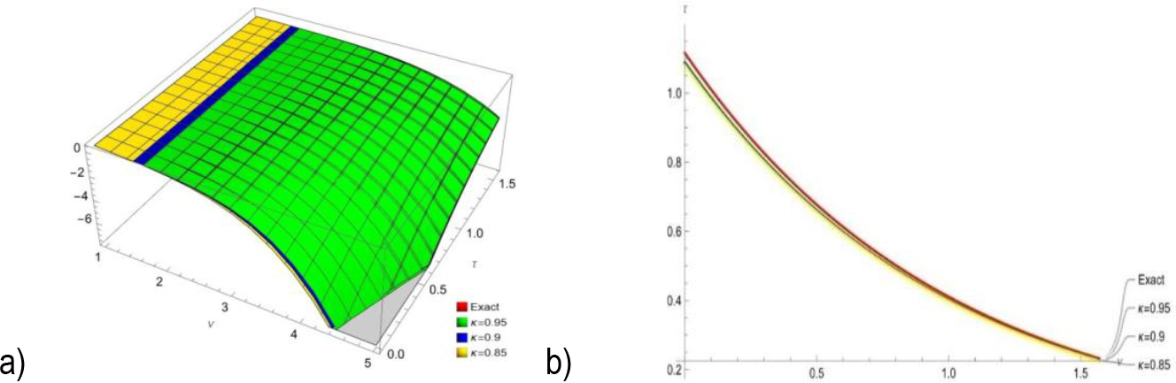
Using a new analytical technique based on ET, this study solves the FCSNLPDEs with ICs; the outcomes of previous approaches are not comparable to those of the present techniques. Multiple parameter values are provided by Equations (8) and (11) in order to give a range of solutions. By allowing the arbitrary parameters to have varying values in the solutions, a range of solutions may be generated. The collected replies are grouped into categories. Additionally, 2D and 3D visual representations are created. These plots may be described using the following details: Figures 1, 2, 3, and 4 show different arrangements of lone waves. Figure 1 was produced for the values in Eq. (8), showing: atκ = 0.95,0.9,0.85., τ = 0.01. This mixture falls within the periodic category, in Eq. (11). Figures 2, 3 and 4 are created using κ = 0.95,0.9,0.85., τ = 0.01.
Fig.1.
(a) Comparing the provided method's 3D representations of the solutions to the exact solutions for Eq. (8), the outcome in comparison to the exact solutions, (b) represent the solutions at κ = 0.95,0.9,0.85
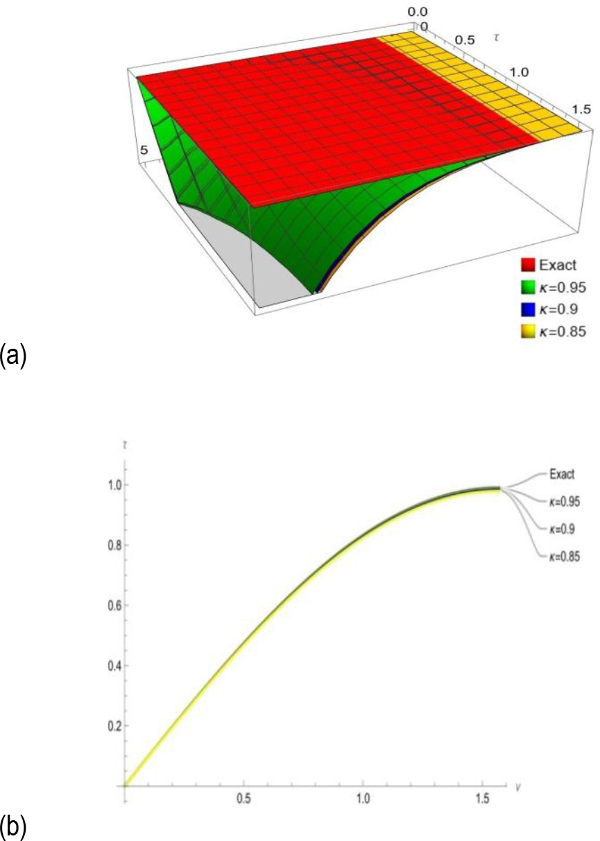
Fig. 2.
(a) Comparing the provided method's 3D representations of the solutions to the exact solutions for Eq. (11), P(υ, ζ, τ) the outcome in comparison to the exact solutions, (b) represent the solutions at κ = 0.95,0.9,0.85
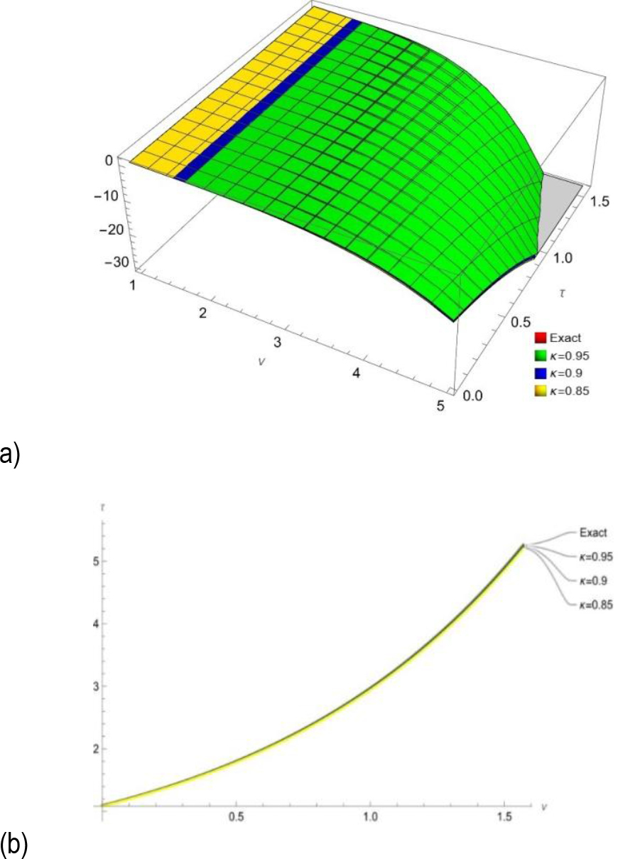
Fig. 3.
(a) Comparing the provided method's 3D representations of the solutions to the exact solutions for Eq. (11), Q(υ, ζ, τ) the outcome in comparison to the exact solutions, (b) represent the solutions at κ = 0.95,0.9,0.85
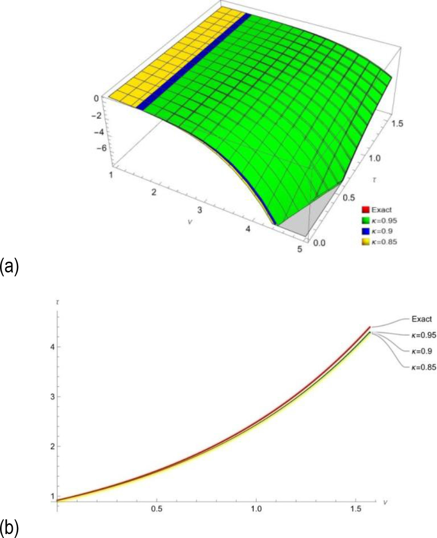
Fig.4.
(a) Comparing the provided method's 3D representations of the solutions to the exact solutions for Eq. (11), K(υ, ζ, τ) the outcome in comparison to the exact solutions, (b) represent the solutions at κ = 0.95,0.9,0.85
The exact solution, which was determined by comparing the values of the exact and approximate solutions of FCSNLPDEs discovered in this problem for various values of the variables,
Tab. 1.
The comparison of the exact and approximate solutions yields the numerical result for example (1)
| τ | υ | κ = 0.85 | κ = 0.9 | κ = 0.95 | Exact | Error | |
|---|---|---|---|---|---|---|---|
| 0 | 0. | 0. | 0. | 0. | 0. | ||
| 0.489578 | 0.491835 | 0.493619 | 0.495025 | 0.00140562 | |||
| P(υ, τ) Q(υ, τ) | 0.01 | 0.847973 | 0.851883 | 0.854974 | 0.857408 | 0.00243461 | |
| 0.979155 | 0.98367 | 0.987239 | 0.99005 | 0.00281124 |
Tab. 2.
The comparison of the exact and approximate solutions yields the numerical result for example (2)
Tab. 3.
The comparison of the exact and approximate solutions yields the numerical result for example (2)
Tab. 4.
The comparison of the exact and approximate solutions yields the numerical result for example (2)
comparing the values of the exact solutions of FCSNLPDEs for various values of the variables,
CONCLUSION
In order to solve FCSNLPDEs using ICs, we created the ET in this study. To demonstrate the usefulness of the proposed method, two examples are provided. It may be possible to handle the solutions in a very basic manner.
The method may be used to tackle a range of initial value problems because to its exceptional ability to solve FCSNLPDEs for various values of fractional orders. Furthermore, 2D and 3D graphs and tables were used to show how the recommended strategy influenced the results. This clearly shows that the new method considerably outperforms the fields when compared to the older methods. In this article we just want to demonstrate the effectiveness of the method discussed and in the near future we will compare this method with other methods to confirm its effectiveness in solving other fractional equations. Also we will consider in future studies the possibility of adapting this approach to other complex systems or fuzzy differential equations. There will be further study done on how to apply this approach to more complex problems, how to integrate it with more sophisticated computer techniques, and how to apply it in the actual world for problems like biological system simulation and epidemic prediction. This advancement creates new avenues for identifying novel solutions to challenging problems in science. Future research will apply the proposed approach to biological simulations and epidemic prediction, extend it to more intricate and stochastic systems, and increase computer efficiency using advanced techniques.