
INTRODUCTION
Ferrofluids are unique types of fluids that exhibit both fluidic and magnetic properties. They are composed of stable colloidal suspensions of single-domain ferromagnetic or ferrimagnetic nanoparticles dispersed in a suitable liquid medium. The magnetic particles typically consist of ferromagnetic metals such as iron, nickel, and cobalt, or ferrimagnetic oxides like magnetite (Fe3O4) and spineltype ferrites. Common carrier liquids include water, ethylene glycol, and various oils. The specific combination of magnetic particles and carrier fluid is chosen based on the intended application of the ferrofluid. Ferrofluids are widely used in sealing, damping, heat transfer, bearings, and sensors. They act as coolants in systems like loudspeakers and transformers, and enhance heat transfer in devices such as heat exchangers. Their use in exclusion seals helps protect sensitive components, making them valuable in robotics, textiles, electronics, and machinery [1, 2].
Due to their vast practical applications, researchers have conducted numerous experimental and theoretical studies on ferrofluids. These studies cover areas such as synthesis and characterization, heat transfer and thermal properties, theoretical modelling and simulation, and industrial applications [3, 4, 5]. Discussing the thermal stability of ferrofluids is equally important as examining their other properties. Understanding thermal stability ensures that ferrofluids can be effectively and safely utilized in current and future technologies.
Thermal stability of ferrofluid in the existence of a vertical magnetic field has been investigated by Finlayson [6]. Schwab et al. examined experimentally the Finlayson’s problem [7]. Thermal stability of ferrofluid depends upon many factors such as density of ferrofluid, gravity acting on ferrofluid, medium of ferrofluid, Coriolis force on ferrofluid and hydrodynamic boundary conditions of ferrofluid. The influence of viscosity variation with magnetic field on thermal convection of ferrofluid has been explored by Sunil et al. [8]. whereas the viscosity variation with temperature field on thermal convection of ferrofluid for general boundary conditions has been investigated by Dhiman and Sharma [9, 10]. The porous medium plays a crucial role in directing geophysically detectable liquids into specific zones for imaging, controlled placement, or chemical treatment. Hence, analyzing the thermal stability of ferrofluids within a saturated porous layer is equally important. Vaidyanathan et al. [11] explored thermoconvective instability in a ferromagnetic fluid saturating a porous medium under the influence of a vertical magnetic field. Since rotation can significantly affect the thermal stability of a fluid layer, Venkatasubramanian and Kaloni [12] examined the impact of rotation on thermo-convective instability in a ferrofluid layer. Many authors have made remarkable contributions to exploring the impact of various parameters on ferrofluid convection (see references [13, 14, 15, 16, 17]).
There are many practical situations where ferrofluids may contain suspended particles. For instance, in industrial settings, ferrofluids are sometimes used as lubricants for machinery, particularly in high-precision equipment like bearings, seals, and pumps. However, in such environments, it is common for the ferrofluid to become contaminated with suspended particles. Therefore, studying ferrofluids with dust particles is equally important. Thermal stability of ferrofluid in the existence of dust particles is studied by Sunil et al. [18]. Sunil et al. [19] explored the impact of viscosity variation with magnetic field on the thermal convection of dusty ferrofluids for the case of free-free boundaries. Sunil et al. [20] conducted a theoretical study on how magnetic field-dependent (MFD) viscosity influences thermal convection in a ferromagnetic fluid saturated porous medium containing dust particles. Sharma and Kumar [21] carried out a theoretical analysis of the combined influence of MFD viscosity and rotation on ferroconvection in a dusty fluid exposed to a uniform transverse magnetic field, whereas Kumar et al. [22] explored the impact of viscosity variation with temperature on the thermal convection of dusty ferrofluids of permeable boundaries. For a detailed understanding of thermal convection in dusty ferrofluids under various effects, one may refer to references [23, 24, 25, 26]. For further insights into related studies involving fluid systems containing dust particles and their significant effects, readers are referred to references [27, 28, 29, 30, 31].
The thermal stability of the liquid is determined by the thermal and hydrodynamic conditions at the surfaces that border it. In past works, fluid boundaries have been mainly either free-free or rigidrigid. However, in many cases boundaries are neither purely free-free nor purely rigid-rigid. For instance, porous structures are used in cooling systems of electronic devices so as to facilitate ferrofluid movement and controlled heat transfer. Magnetic seals in rotating machinery consist of field-permeable membranes that maintain fluid position while allowing for fluid exchange and pressure fluctuations. For example, targeted drug delivery and hyperthermia treatment require ferrofluids to pass through semi-permeable biological membranes. Also heat exchangers, magnetic field-controlled filtration systems, ferrofluid-based microfluidic devices and aerospace thermal management all rely on boundary permeability for effective thermal convection. Siddheshwar [32] has documented the convective instability of ferromagnetic fluids confined by fluid-permeable and magnetically active boundaries. More recently, Nanjundappa et al. [26] explored penetrative ferro-thermal convection (FTC) driven by internal heating in a porous layer saturated with ferrofluid, considering various temperature, velocity, and magnetic potential boundary conditions. Additionally, Surya [33] examined convective instability of a liquid layer with permeable boundaries under the influence of variable gravitational force.
To the best of our knowledge, no prior studies have examined the combined effects of viscosity variation with magnetic fields and fluid-permeable magnetic boundary surfaces on the thermal convection of ferrofluids containing dust particles. This research is motivated by this gap in the literature. The study will provide different insights on how thermal convection can be optimized for various engineering applications such as electronics cooling, aerospace systems, biomedical technologies and environmental engineering through dust particles effects on it and variation of viscosity with magnetic field and fluid – permeable magnetic boundaries.
RESEARCH METHODOLOGY
The analytical investigation of convective instability in a dusty ferromagnetic fluid layer considering magnetic field-dependent viscosity and fluid-permeable, magnetically active boundaries under a uniform transverse magnetic field follows a structured approach aligned with the objectives of the study. A brief overview of the methodology is presented below as per the defined sections.
. Fundamental Equations of the Problem
This phase includes recognizing and developing the core equations that govern the problem. These equations may be based on physical laws or derived from mathematical models.
. Basic State
After establishing the fundamental equations, the system’s basic state is identified. The system is considered to be in this basic state when there is no fluid motion in its initial condition.
. Perturbation
Perturbations refer to small disturbances or deviations from the basic state that are introduced into the system. These disturbances enable the examination of the system’s stability and behavior under different conditions [34].
. Linear Analysis
To identify the instability threshold for an dusty ferromagnetic fluid during thermal convection, linear analysis specifically using normal mode analysis as described by Chandrasekhar [34] to create an eigenvalue problem offers valuable insights into the fundamental physics of thermal convection.
. Normal Mode Analysis
Normal mode analysis is utilized to reduce the system of partial differential equations into an eigenvalue problem, which allows for a systematic examination of the stability of the system.
. Non-dimensionalize the System of Equations
The governing equations of the system are non-dimensionalized to simplify the analysis and eliminate any reliance on specific units of measurement. Scaling factors are used to non-dimensionalize the perturbed equations.
MATHEMATICAL MODELLING
Consider a static layer of ferromagnetic fluid with a finite vertical thickness d and an infinite horizontal extent, heated from below, and containing dust particles. This fluid layer is subjected to a uniform vertical magnetic field H and experiences a gravitational force represented by and this system is confined between two horizontal fluid-permeable magnetic boundaries (as depicted in Fig. 1)
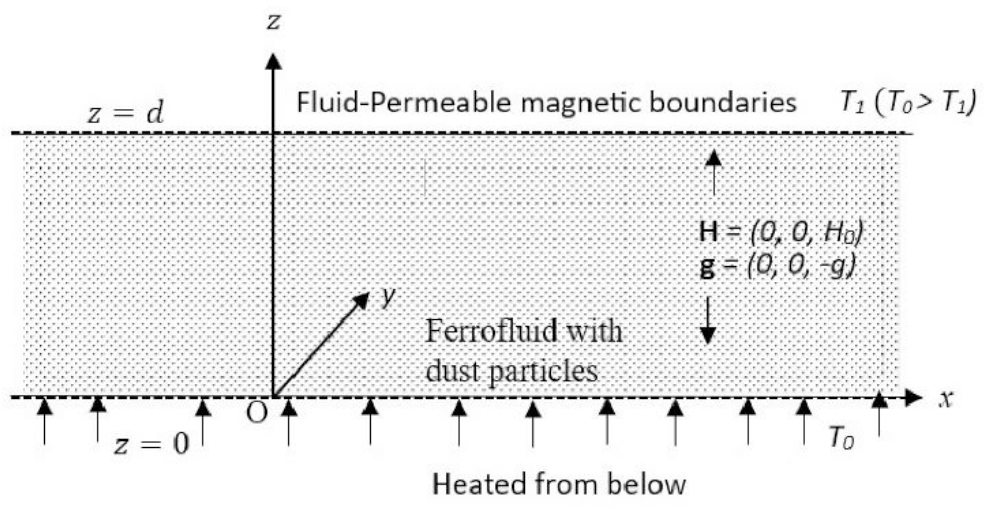
We assume the fluid is incompressible, electrically non-conduc-tive, and has a viscosity depend upon the magnetic field, expressed as μ = μ1(δ.B + 1) [35]. The fluid's viscosity when the magnetic field is zero is μ1, the isotropic coefficient of viscosity change is δ, and the magnetic induction is represented by B. For the model described, the governing equations under the Boussinesq approxi-mation are provided by [6, 19]:
The equation of state for density is
In the aforementioned equations: q represents the ferrofluid’s velocity, q indicates the dust particles’ velocity, pertains to pressure, ρ corresponds to density, Nd signifies the number density of the dust particles, M stands for magnetization, B represents magnetic induction, T is the temperature, CH,V characterizes the specific heat at constant magnetic field and volume, Cpt indicates the specific heat of dust particles, K1 designates the thermal conductivity, α represents the coefficient of thermal expansion, and K = 6πμr signifies the Stokes drag coefficient, where r represents the radius of the dust particle. Additionally, ρ0 and μ0 correspond to the density and magnetic permeability at the reference temperature.
The buoyant force acting on the dust particles is neglected [18, 23, 26]. It is further assumed that the spacing between the particles is much larger than their diameters, allowing inter-particle interactions to be disregarded. The influence of gravity, pressure, and viscous forces on the particles is assumed to be negligibly small and is thus omitted from consideration. An additional force term with this opposite direction must be included in the particles' equation of motion, because the force applied by the ferrofluid on the dust particles is equal in magnitude but opposite in direction to the force exerted by the dust particles on the ferrofluid. Let mNd denote the mass of dust particles per unit volume; the motion and continuity equations for the dust particles, under these assumptions, are given as follows [19, 22]:
Due to assumption that fluid is electrically non-conductive, the equations of Maxwell in the case where displacement current is absent for a non-conductive fluid can be stated as follows [6]:
andThus, from equations (7) and (8), we get
The alignment of magnetization is governed by both the mag-netic field's strength and temperature, resulting in the following re-lationship
andWhere M0 is the magnetization when temperature is T0 and magnetic field is H0, while
represents the pyromagnetic coefficient and magnetic susceptibility respectively.Equations (1) to (11) are solved for zero flow at base state and thus the basic state solutions are given by
12
Further following Finlayson [6] perturbations are added to initial basic state as:
Where the variables
represent infinitesimal disturbances in density, pressure, velocity of ferrofluid, velocity of dust particles, magnetic field intensity, magnetization and temperature, respectively.On introducing equation (13) into equations (1) to (11) and applying the basic state solutions, we derive the linearized perturbation equations in the form.
Here ρC1 = μ0H0K2 + ρ0CH,V,
Here we have considered that βdK2 < <(χ + 1)H0. (Finlay-son [6]).
Now, eliminating p′, u′, v′ between equations (15)–(17) using equation (14), we get
whereAlso, from equations (19) and (20), we have
Now, following normal mode analysis assuming that all quanti-ties characterizing the perturbation depend on t, x, y, and z in the form
In this context, we have wave numbers represented as kx1and ky1 for the x and y directions, respectively. Additionally, n denotes the growth rate, and k is defined as the magnitude of the resultant wave number, calculated as the square root of the sum of the squares of kx1 and ky1 and using non dimensional parameters:
A real independent variable in the range 0 ≤ ≤ 1 is used in the aforementioned equations. Here, the square of the wave number is represented by a2, while differentiation with respect to z is shown by
From a physical standpoint, equations (24) to (26) define an eigenvalue problem for R, which governs ferromagnetic convection within a ferrofluid layer containing dust particles. In these equations, w represents the vertical velocity, θ indicates the temperature, and ϕ denotes the amplitude of the magnetic potential. Since M2 is of a very small magnitude (on the order of 10−6) [6], its influence is negligible for further analysis, allowing equation (25) to be simplified as.
For the scenario of stationary convection, setting ω = 0 simplifies the eigenvalue problem into the following form:
Since the ferrofluid layer is confined between two thermally conducting and fluid-permeable magnetic surfaces. Hence, we use the following fluid-permeable magnetic boundaries condition as proposed by ([6, 32, 36, 37]):
where Das is the slip-D'Arcy number and χ is the magnetic susceptibility.MATHEMATICAL ANALYSIS
The non-dimensionalized linear ODEs (28) to (30) along with boundary conditions (31) form the eigen value problem with as Rayleigh number. To determine the Rayleigh number for the given boundary conditions (31), we will employ a single-term Galerkin method. Let’s consider a single term in the expansions of w, θ, and ϕ as follows:
Here, A11, B11, and C11are constants, and w1(z), θ1(z), and ϕ1(z) are appropriately selected trial functions that satisfy the necessary boundary conditions (31). By replacing w, θ, and ϕ with their respective expressions in equations (28) to (30), then multiplying each resulting equation by w1(z), θ1(z), and ϕ1(z) accordingly, and integrating by parts the necessary number of times while applying the boundary conditions, we derive three homogeneous equations in A11, B11, and C11. The coefficients of these equations are expressed as definite integrals. This system can be expressed in matrix form as follows:
where,For simplicity, the subscript 1 is omitted, and the functions w1(z), θ1(z), and ϕ1(z) are henceforth denoted as w, θ, and ϕ respectively.
For a non-trivial solution to occur, the determinant of the coefficient matrix must be zero. This results in the following expression, which establishes a first-order relationship between the Rayleigh number R and the wave number a.
Let us now select the following trial functions that satisfy the specified boundary conditions.
The initially proposed trial function for the magnetic potential, denoted by ϕ, does not meet the boundary conditions given in equation (31). To resolve this inconsistency, the boundary residual method, as described by Finlayson [6], is applied to the function ϕ.
By applying these trial functions to the integrals A1 through A6, we derive the following formula for Rayleigh number as
35
Using MATLAB R2023a software, the square of the critical wave number xc is determined by finding the positive roots of the equation
Also, we have the following formula for the magnetic Rayleigh number N for significantly large values of M1derived from expression (35) utilizing Finlayson [6] analysis.
which stand for the magnetic mechanism that functions when buoyancy effects are not present.RESULTS AND DISCUSSION
This study explores the convective instability of a dusty ferromagnetic fluid, incorporating the effects of viscosity that depend on the magnetic field. The system is analyzed within a Rayleigh-Bènard configuration, where the fluid is contained between permeable boundaries that are also magnetically active. Additionally,the setup is subject to a uniform transverse magnetic field. Given the complexity of the boundary conditions, the Galerkin method was employed to calculate the critical eigenvalue. These findings can contribute to better control of instability in engineering systems and enhance the efficiency of applications where stability and precise thermal regulation are essential.
In the present analysis, the nonlinearity of the magnetization parameter M3 is considered to vary from 0 to 25, as suggested by Finlayson [6]. The MFD viscosity parameter δ ranges from 0 to 0.09, as per the work of Prakash et al. [14]. The dust particle parameter h1 is taken to vary between 1 and 9, following the suggestion of Sunil et al. [18]. Furthermore, the magnetic susceptibility of boundaries and the permeability parameter of boundaries χ are assumed to range from 100 to 106 and from 0 to ∞, respectively, as suggested by Siddheshwar [32].
First, we discuss the accuracy of the results presented in this study. For the case of ordinary fluid, in the absence of a magnetic parameter (M1 = 0 and M3 = 0), χ → ∞ and without dust particles (h1 = 1), the critical Rayleigh number (Rc) and wave number
Also, Tab. 1 provide a qualitative comparison of the numerical results computed at χ → ∞, without dust particle (h1 = 1), M3 = 10, M1 = 1,5 for the case of free-free and rigid-rigid boundaries with Dhiman [10]. The table clearly shows that our results align exceptionally well with previously published data, confirming the accuracy of our numerical procedure.
Tab. 1.
Comparison of Values from the Present Study with Existing Studies
| Free-Free | Rigid-Rigid | |||
|---|---|---|---|---|
| Present Study | Dhiman [10] | Present Study | Dhiman [10] | |
| M1 = 1 | 360.0088 (5.4644) | 342.52 (5.174) | 913.1268 (10.2291) | 889.15 (9.921) |
| M1 = 5 | 126.5677 (5.8260) | 116.49 (5.319) | 313.1211 (10.5816) | 299.56 (10.06) |
Tab. 2 presented the numerical values of critical magnetic Rayleigh number (Nc) and square of critical wave number
Tab. 2.
Variation of critical magnetic Rayleigh numbers Nc with M3, χ and δ at fixed h1 = 3 and Das = 1
Fig. 2 depict the variation of critical magnetic Rayleigh numbers Nc versus χ with different values of M3 and fixed values of δ, h1 and Das. From Fig. 2 and numerical values of critical magnetic Rayleigh numbers Nc presented in Tab. 3 we can observe that critical magnetic Rayleigh numbers increases for increasing values of χ, which yields that χ has stabilizing effect on the system. This stabilizing effect of χ directly depend upon M3, χ has strong stabilizing effect for smaller values of M3 as compare to larger values of M3. Also from Tab.3 we can observe that the critical wave number increases as χ increases which indicate that χ reduces the size of convection cell.
Tab. 3.
Variation of critical magnetic Rayleigh numbers Nc with h1, M3 and Das at fixed χ = 10 and δ = 0.03
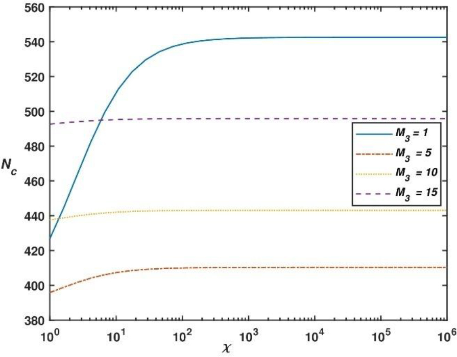
Fig. 3 epict the variation of critical magnetic Rayleigh numbers Nc versus Das with different values of and fixed values of M3, h1 and χ. From Fig. 3 and numerical values of critical magnetic Rayleigh numbers Nc presented in Tab. 4 we can observe that critical magnetic Rayleigh numbers increases for increasing values of Das, which yields that Das has stabilizing effect on the system. Also we can conclude that (Nc)Free ≤ (Nc)Permeable ≤ (Nc)Rigid. Because (Nc)Free and (Nc)Rigid can be acquired from (Nc)Permeble in the limit Das → 0 and ∞ respectively. Therefore the equality sign in (Nc)Free ≤ (Nc)Permeable ≤ (Nc)Rigid is understandable. This analysis effectively demonstrates the connection between the results for free-free and rigidrigid boundary conditions. This behavior arises because free boundaries impose minimal resistance to fluid motion near the surfaces, allowing the temperature gradient to drive convection more easily. As a result, the fluid becomes more responsive to instabilities, leading to a lower critical magnetic Rayleigh number and an earlier onset of convection compared to the case with rigid boundaries. Further, it is evident from Tab. 4 that the critical wave number increases as Das increases which indicate that Das reduces the size of convection cell.
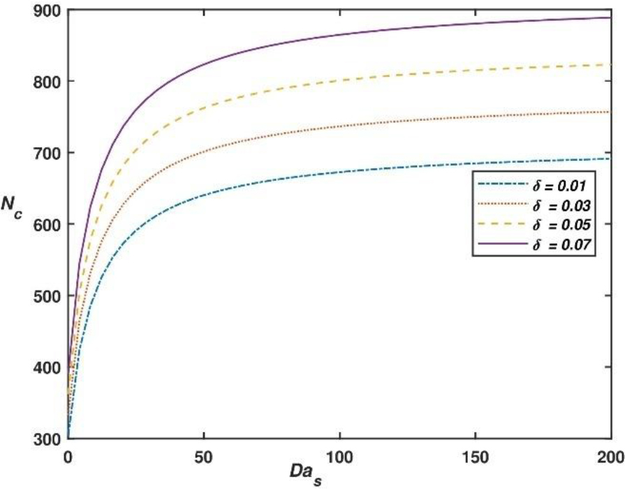
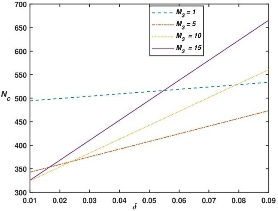
Fig. 4 depict the variation of critical magnetic Rayleigh numbers Nc versus δ with different values of M3 and fixed values of χ, h1 and Das. From Fig. 3, Fig. 4, Fig. 5, Fig. 7 and numerical values of critical magnetic Rayleigh numbers Nc presented in Tab. 3 we can observe that critical magnetic Rayleigh numbers increases for increasing values of δ, which yields that δ has stabilizing effect on the system. This is consistent with the physical understanding that higher viscosity suppresses disturbances and restricts fluid movement, resulting in a delayed onset of convection. Also, it is noted from table Tab. 3 that the critical wave number has no influence of MFD viscosity δ, i.e. size of convection cell is independent of MFD viscosity δ.
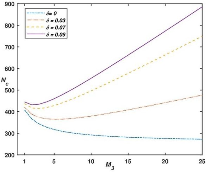
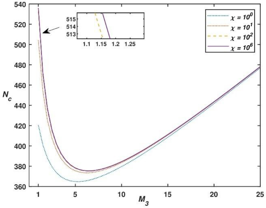
The behavior of the critical magnetic Rayleigh number Nc as a function of M3 is illustrated in Fig. 6 for several values of χ, while keeping M3, h1 and δ constant. Similarly, Fig. 7 depicts the relationship between Nc and M3 for different values of δ, with h1, M3, and χ held fixed. The critical magnetic Rayleigh number Nc initially decreases for increasing values of M3, but after a certain value of M3, it increases for increasing values of M3, as shown by Fig. 2, Fig. 4, Fig. 6, Fig. 7 and Tab. 2 as well as Tab. 3. This destabilizing or stabilizing effect of M3 varies upon the value of. The destabilizing effect range of M3is larger for small values of than it is at large values of. From Tab. 2 and Tab. 3 it is observed that critical wave number reduces with raise in M3 which means that M3 increases the size of convection cell.
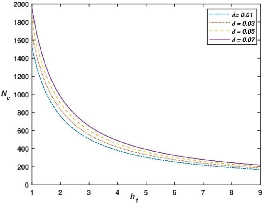
The behavior of the critical magnetic Rayleigh number Nc as a function of dust particles parameter h1 is illustrated in Fig. 5 for several values of, while keeping h1, M3, and χ constant. From Fig. 2 and numerical values of critical magnetic Rayleigh numbers Nc presented in table Tab. 2 we can observe that critical magnetic Rayleigh numbers decreases for increasing values of h1, which shows that h1 has destabilizing effect on the system as the overall heat capacity of the fluid increases due to the additional contribution from the dust particles. Moreover Tab. 2 demonstrates that the critical wave number does not depend on the parameter h1 of dust particles, meaning that the size of the convection cell is not affected by dust particles parameter h1.
CONCLUSION
For a Rayleigh-Bénard situation between fluid-permeable, magnetic boundaries, we investigate the impact of dust particles and viscosity variation with magnetic field on the convective instability of a ferro magnetic fluid layer using the single term Galerkin technique for stationary mode of convection. The main conclusion from our research can be summarized as follows:
– The parameters of fluid permeable, magnetic boundaries and MFD viscosity parameter delay the initiation of onset of convection which indicate their stabilizing effect.
– Dust particles parameter h1 initiate the initiation of onset of convection which indicate their destabilizing effect.
– Measure of nonlinearity of magnetization M3 exhibits a destabilizing effect, but beyond a certain threshold, it switches to a stabilizing effect within the system.
– The size of cells formed at the initiation of convection narrows with a raise in the parameter of permeable magnetic boundaries.
– The size of cells formed at the initiation of convection widens with a raise in the measure of nonlinearity of magnetization 3.
– The dust particles parameter and MFD viscosity has no effect on the size of cell formed at the initiation of convection.
These discoveries advance our knowledge of the variables affecting convection of ferrofluid and offer useful data for a number of disciplines, including fluid dynamics and geophysics. Additional investigation in this field may clarify our understanding of convection phenomena and examine the practical consequences of these results.