1. INTRODUCTION

There are several system disturbances, which can lead to in-stability or poor performance. Therefore, several anti-disturbance control techniques have been developed by researchers to enhance the anti-disturbance performance of systems. For example, [1] developed a H_∞ control with an observer for eliminating a norm-bounded disturbance and a disturbance defined by an exogenous system on an aircraft model. [2] proposed a methodology for Markovian jump systems under the influence of multiple disturbances. A sliding mode observer and a feedback control law based on the backstepping method were employed in [3] for flexible spacecraft systems. [4] designed a flight controller for a helicopter system using a disturbance observer and a backstepping controller. A disturbance rejection control method was proposed by [5] using H_∞ control and the equivalent input disturbance method for an aircraft system. The equivalent input disturbance method was employed in [6] to estimate exogenous perturbations with the Lyapunov-based state feedback control law and in [7], authors improved the disturbance estimation performance of modelling equivalent input perturbations for a missile autopilot design. [8] developed a sliding mode controller in conjunction with a disturbance observer for a quadrotor helicopter where the disturbance observer estimates the impact of persistent and gradually changing disturbances. [9] suggested a methodology combining a sliding mode controller and a dual disturbance observer to manage spacecraft position and attitude dynamics, where the dual disturbance observer based controller attenuates both the external disturbances characterized by the exogenous model and the bounded disturbances. The helicopter slung load system was governed by a composite anti-disturbance model reference controller, which ensured asymptotic stability and L₂ − L_∞ performance in [10]. A composite control strategy comprising a disturbance observer and a robust controller was designed by [11] to handle with multiple disturbances in a rigid spacecraft system, aiming to achieve anti-disturbance performance. A hybrid control approach was presented in [12] for Markovian jump systems affected by multiple disturbances. This approach specifically addresses an energy-bounded disturbance alongside an event-triggered sinusoidal disturbance characterized by unknown frequencies and amplitudes. An anti-disturbance control was designed in [13] which tackles the challenges of finite-time boundedness and disturbance rejection in takagi-sugeno fuzzy networked systems, particularly those susceptible to actuator faults, linear fractional uncertainties, and multiple disturbances. In [14], researchers investigate a distributed extended state observer design and a dual-side dynamic event-triggered output feedback anti-disturbance control strategy for interconnected systems facing quantization issues and multi-source disturbances.

In another research domain, there has been a notable rise in interest regarding the analysis of stability and design of controllers for switched systems [15], because switched systems find wide-ranging applications across various industries, including but not limited to the automotive industry, aviation, air traffic control systems, switching power converters, and so on [16]. At present, numerous significant findings have emerged regarding the stability and control synthesis of switched systems. Generally, the most prevalent approaches to designing switching laws involve state- and time-dependent switching rules [17,18,19]. A state-dependent switching law refers to a switching function that depends on the system state. Even though individual subsystems exhibit instability, the overall stability of the switched system can be preserved. Nevertheless, the chattering phenomenon [20] may be revealed because any dwell-time constraint cannot be guaranteed between switching instants. A few examples of dwell-time switching laws [21, 22, 23] which are formulated based on time-dependent rules. The amplitude changes in switching controllers may lead to control bumps, negatively affecting transient performance and potentially causing instability. This issue was addressed in [24,25], where the authors proposed an H_∞ bumpless transfer controller specifically designed for switched interval type-2 (IT2) fuzzy systems. A fault tolerance and anti-disturbance attenuation using a two-dimensional modified repetitive control system was invetigated in [26] for switched fuzzy systems with multiple disturbances.

Various disturbances occur during flight, which can significantly impact the performance of aero-engine systems. Consequently, developing anti-disturbance controllers for these systems is imperative. However, the challenge of implementing effective disturbance-rejection control in aero-engine systems especially in the presence of multiple disturbances remains largely unaddressed. This gap in the existing literature serves as the main motivation behind our study. By focusing on the unique challenges faced by aero-engine systems, we aim to contribute a robust framework for designing anti-disturbance controllers that can effectively manage multiple disturbances. Our research not only addresses this critical need but also provides innovative solutions that enhance the stability and performance of aero-engine systems in dynamic flight conditions. This work lays the groundwork for future advancements in control strategies within the aerospace industry, promoting greater safety and efficiency in aircraft operations. In this paper, we address the challenge of composite disturbance-rejection ℋ₂ control for switched systems. Many control systems encounter significant challenges from external disturbances that can compromise operational stability. Traditional control strategies often struggle to maintain performance under such conditions, leading to increased instability and inefficiency. To address these issues, developing an anti-disturbance approach is essential for ensuring consistent performance and reliability. The anti-disturbance switched ℋ₂ control method specifically enhances system performance and optimizes operational efficiency. We propose a composite anti-disturbance control scheme to effectively manage multiple disturbances. The need for effective control of time-varying systems, particularly those subjected to external disturbances, has led to the development of advanced control strategies. In this context, our composite anti-disturbance control approach integrates disturbance observer-based control with robust switching strategies, offering superior disturbance rejection compared to traditional methods. A key advantage of our method is the use of a state-dependent switching law, which makes the system highly adaptable to time-varying dynamics—a significant improvement over static or less adaptive control schemes. Additionally, the integration of an ℋ₂ based controller ensures optimal tracking performance. When combined with the disturbance observer, it outperforms standard ℋ₂ methods, providing better tracking accuracy while maintaining comparable levels of robustness. The proposed design also tackles common challenges in switching systems by carefully managing dwell times and switching conditions, ensuring both stability and high performance without typical drawbacks like chattering. The key contributions of this work are as follows: We propose a disturbance observer-based control approach and a switched state feedback ℋ₂ control method for a class of switched systems experiencing multiple disturbances. Here, the disturbance observer is designed to estimate the external disturbances described by an exogenous system. The outputs of the disturbance observer and the switched ℋ₂ state feedback controller are integrated to form a composite anti-disturbance switched controller. We present conditions, formulated as LMIs, that guarantee robust stability of the closed-loop system while maintaining the specified ℋ₂-norm. A growing number of articles has focused on control problems in aero-engine systems, highlighting the significance of this area in engineering. To demonstrate the effectiveness of our proposed composite anti-disturbance control scheme, we apply it to an aero-engine system. We achieve stability of the controlled aero-engine system by applying minimum dwell-time theory.

The structure of this paper is as follows: In the subsequent section, we provide the preliminaries and problem formulation. We then detail a composite anti-disturbance ℋ₂ control scheme using LMIs in Section 3. Application of the proposed control approach to an aero-engine model is detailed in Section 4. Following this, simulation results are presented in the subsequent section to show the effectiveness of the developed control scheme. Lastly, the conclusions of this paper are given.

Notation: The function Tr(.) represents the trace operation for square matrices. He{A} = A + A′ is called He{.}. P are symmetric matrices and P > 0 (≥ 0) indicates positive definiteness (semi-definiteness). A symmetric matrix of the form PQQ′P is denoted as PQ*P . We denote ℝⁿ as the n-dimensional Euclidean space and ℝ^p×q as the set of all p × q real matrices. Additionally, ℕ denotes the set of natural numbers.

2. PRELIMINARIES AND PROBLEM FORMULATION

Consider a dynamic system described by:

In this paper, the disturbance observer is formulated as:

The disturbance estimation error can be calculated as

Combining (2), (3) and (5), we have

Thus, the output is given such:

Therefore, using (6) and (7) with (1) the augmented system is obtained

Switched System Case

A nominal linear switching system emerges as a special case of system (1),

(9)

dxθdθ=Aξθθxθ+Bξθθuθ+δ1θ            +Bw,ξθθδ2θ,

where the switching rule function ξ(θ) defined for θ ≥ 0. ξ(θ) takes values from 1, …, M, here M is the time-varying subsystems’ number. Assuming that the system matrices of (9) are contained within the collective polytopes ζ_i(θ) of the subsystems:

(10)

ζθ=∪i=1Mζiθ

where the definition of ζ_i(θ) is as follows:

(11)

ζiθ=AiθBiθBw,iθ=∑j=1Nκjθζij,

where

(12)

∑j=1Nκjθ=1,κjθ≥0, θ≥0

and

(13)

ζij=AijBu,ijBw,ij

Remark 1. In the preceding definition, the sub-polytopes are indexed by the variable i, which ranges from 1 to M. Additionally, j indexes the vertices of the corresponding sub-polytope, with each sub-polytope assumed to possess N vertices. The convex combinations of these vertices give the matrices of the related sub-system. It is assumed that the sub-polytopes share some common regions and that the rates of change with respect to time for the polytopic coordinates κ_j(θ), ∀ j = 1,…,N, are bounded.

Then, the external disturbance, δ₁(θ) in (2) defined as:

(14)

w˙θ=Eξθθwθ+Fξθθδ3θδ1θ=Gξθθwθ

Therefore, the disturbance observer is formulated such

(15)

v˙θ=Eξθθ+LξθBξθθGξθθw^θ   −LξθAξθθxθ+Bξθθuθw^θ=vθ−Lξθxθδ1^θ=Gξθθw^θ

and the state feedback control law is

(16)

uθ=Kξθxθ−δ1^θ

Combining (14), (15) and the disturbance estimation error e_w(θ) = w(θ) − ŵ(θ), we have

(17)

e˙wθ=Eξθθ+LξθBξθθGξθθewθ   +LξθBw,ξθθδ2θ+Fξθθδ3θ

Finally, the augmented system is obtained based on the system in (9) and the system output

(18)

zθ=C1,ξθθxθ+C2,ξθθewθ,x˜˙θ=A˜ξθx˜θ+B˜ξθδθzθ=C˜ξθx˜θ

where

x˜θ=x′θ, e′θ′,δθ=δ2′θ,δ3′θ′A˜ξθθ=Aξθθ+BξθθKξθBξθθGξθθ0Eξθθ+LξθBξθθGξθθ,B˜w,ξθθ=Bw,ξθθ0LξθBw,ξθθFξθθ,C˜ξθθ=C1,ξθθC2,ξθθ

The augmented system parameters are uncertain and presumed to reside in the union of the subsystems’ polytopes as in (10). For simplicity, the notation θ will be dropped in the following sections.

Remark 2. In this paper, we employ a state-dependent switching law, as given in [18], which adheres to a dwell time constraint with a specified dwell time. This approach effectively manages the switching between different modes, thereby enhancing the overall stability and performance of the control system.

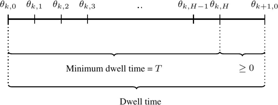
Definition 1. Throughout this paper, we adopt the assumption of a minimum dwell time constraint on the switching signal ξ(θ). This constraint implies that if the minimum dwell time is denoted by T, and the system’s switching instants are represented as (θ₁,θ₂,…), then it holds that θ_k+1 − θ_k ≥ T ∀ k ≥ 1. Here, we define the time instants θ_k,h : = θ_k + hT/H, where h ranges from 0 to H, and θ_k,0: = θ_k, ∀ k. Consequently, the minimum dwell time constraint T ensures that θ_k,H ≤ θ_k+1,0. This definition is explained in Fig. 1.

Fig. 1.

Splitting the minimum dwell-time into H equal segments

3. COMPOSITE ANTI-DISTURBANCE CONTROL SCHEME

ℋ₂ control design is often adopted to deal with the transient performance of closed-loop systems. The ℋ₂-norm in terms of LMIs can be defined as in the following lemma.

Lemma 1. (ℋ₂-norm [27]) Given that A in the system (1) is Hurwitz and the corresponding transfer function is represented by G(s) = C(sI − A)⁻¹ B + D, the following statements are equivalent:

Lemma 2. For the system (8), the following statements are equivalent to Lemma 1;

there exist symmetric matrices, Q > 0, P > 0 and Z such that

Given positive scalars α and β, if there exist matrices X and Y, along with symmetric matrices Q > 0, P > 0, and Z, such that

Proof: Denoting P = diag(P₁, P₂) and replacing the system matrices in Lemma 1(ii) with the augmented system matrices (8), then the following equivalent conditions are obtained:

Denoting P˜=diagP1−1,I,I and P¯=diagP1−1,I,I,I , multiplying (19) and (20) by respectively P˜ and P¯ from both sides, then the conditions in Lemma 2(ii) are obtained.

The proof of Lemma 2(ii) relies on applying the Finsler lemma in conjunction with Lemma 2(i). Also, multiplying Lemma 2(ii) the left by ϒ and from the right ϒ′ the condition of Lemma 2(i) are obtained, where:

For the switched linear time-varying (LTV) system (18), the conditions in Lemma 2(i) can be rewritten as follows:

As in [28], positive-definite Lyapunov matrices dependent on time and parameters, Qξθjθ∈Q1jθ, …,QMjθ and Pξθjθ∈P1j(θ),…,PMjθ , are defined as:

Theorem 1. If a scalar T > 0 is given, and there exist matrices Si,hj , Ri,hj , as well as positive-definite symmetric matrices Z, Pi,hj , and Qi,hj that satisfy the following LMIs minimization program ∀ i = 1, … , M and j = 1,…,N:

minimise Tr(Z)

subject to

Then it guarantees that the closed-loop system (18) exhibits global stability, while the closed-loop ℋ₂-gain from d to z is maintained at TrZ or less for any switching rule with a dwell-time equal to or greater than T.

Based on the above conditions and Lyapunov matrices, the following theorem is defined to provide solutions to the composite anti-disturbance control problem within the framework of the switched linear time-varying (LTV) system (18).

It is notable that prior to the initial switching event, the Lyapunov function experiences a decrease due to the conditions (23c). This indicates that the control strategy effectively preserves the Lyapunov function in the absence of switching, ensuring system stability and performance. Throughout the time span θ_k ≤ θ ≤ θ_k + T, conditions (23a, 23b) derived from (21 and 22) ensure a consistent monotonous decrease in the Lyapunov function. Following this, conditions (23c) ensure the continuous decrease of V(θ, x) after θ_k + T and before the subsequent switching event. The non-increasing property of the Lyapunov function between any two arbitrary switching events is guaranteed by the conditions (23d).

Remark 3. According to Theorem 1, the state-feedback gains Kijθ and the disturbance observer gains Lijθ vary over time and depend on vertices. Nonetheless, these gains are often impractical for real-world use. Instead of those, time-invariant state-feedback gains and disturbance observer gains are often preferred. Therefore, the following theorem is formulated by using the conditions in Lemma 2(ii).

Remark 4. The computational complexity is given by N(3MH + 3M − 1), where N represents the number of vertices, M is the number of subsystems, and H is the number of time instants. From this equation, we can conclude that both N and M contribute linearly to the overall computational complexity. This implies that if either the number of vertices or the number of sub-systems increases, the computational effort will increase proportionately.

Theorem 2. For the given scalars T > 0, α > 0, and β > 0, if there are matrices Si,hj , Ri,hj , Xi,hj , Yi,hj , and positive-definite symmetric matrices Z, Pi,hj , and Qi,hj ; ∀ i = 1, … , M and j = 1, … , N that satisfy the following LMI minimization conditions:

minimise Tr(Z)

subject to

Remark 5. Theorem 2 provides vertex-dependent and time-varying state-feedback gains, Kijθ , and disturbance observer gains, Lijθ . However, if Si,hj , Yi,hj , Xi,hj , and Ri,hj are selected independently of h and j, then these gains become time-invariant. They can be computed as Ki=SiYi−1 and Li=Xi−1Ri .

Remark 6. The ℋ₂ controller ensures optimal tracking performance by minimizing the quadratic cost function associated with tracking error and control effort. Integrating a disturbance observer enhances this performance by compensating for disturbances, improving tracking accuracy and overall system effectiveness. This combination allows the controller to adapt to varying disturbance levels, making it more versatile in handling unpredictable real-world scenarios.

It is important to note that as the size of the LMIs increases, there is a potential for a greater computational burden. Larger LMIs can introduce higher complexity in the numerical solving process, requiring more computational resources and time. However, advancements in modern computing technology have made it feasible to manage these challenges effectively. Furthermore, this computational complexity primarily arises during the initial design phase. Once the control strategies are established, the size of the LMIs becomes less significant, as they do not affect real-time implementation. Consequently, the initial investment in computational resources can yield robust and efficient control solutions that perform effectively in practice.

4. APPLICATION TO AERO-ENGINE MODEL

In this section, we showcase the implementation of the proposed anti-disturbance control scheme on the speed control system of the GE-90 aero-engine. We begin by presenting the GE-90 aero-engine model and then delve into the discussion of simulation results.

Aero-engine model

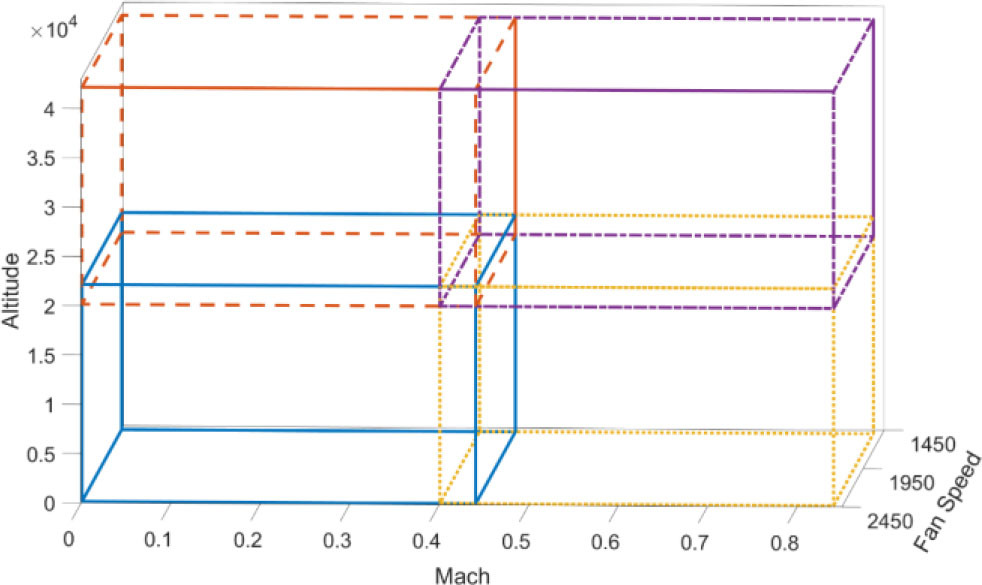
The aero-engine is comprised of essential components such as a combustion chamber, turbine, and compressor. Both the compressor and turbine feature high-pressure and low-pressure stages with rotating blades. The high-pressure compressor and turbine are concentrically aligned via a separate shaft, while the low-pressure compressor and turbine, along with the fan, rotate synchronously. Positioned at the inlet, the fan facilitates airflow, and a variable bleed valve is employed to extract gas from the core. Additionally, variable stator vanes aid in reducing flow separation within the compressor blades. Further details can be found in [29, 30]. The aero-engine has complex and highly non-linear dynamics. In the literature, different models of aero-engines have been developed. For this study we will use an LPV model of aero-engine (GE-90) which has been proposed by [29]. The altitude is normalized by 10000 and the fan speed by 3000. An LPV model of the uncertain state-space presentation is

(30)

ΔN˙fΔN˙c=Am,h,fΔNfΔNc+Bm,h,fΔWF+δ1+Bwδ2

and the external disturbance system

(31)

w˙θ=Eξθwθ+Fξθδ3θδ1θ=Gξθwθ

where m, h and f denote the Mach number, altitude and fan speed respectively. ΔN_f = N_f − N_f0 is the fan speed increment, ΔN_c = N_c − N_c0 is the core speed increment and ΔW_F = W_F − W_F0 is the fuel flow increment. Also, δ₁ is the external disturbance, δ₂ = te^−t is another disturbance and δ₃ = te^−t is an additional disturbance which results from the perturbations and uncertainties in the external disturbance. The engine pressure ratio (EPR) increment is

EPR=CΔNfΔNc

Here, the Mach number, the altitude and the fan speed parameters vary between [0 – 0.84], [0 – 42000] and [1497 – 2432] respectively. Using these parameters, the system has been partitioned into four intersecting cells, as illustrated in Fig. 2. Model parameters can be obtained for each vertex and cell according to [23].

Fig. 2.

The cell divisions of the parameters

Then, using LPV model in (30) with vertices of each cell, the switch system matrices Aij , Bij and Cij in (9) are obtained and the matrices Bw,ij , Eij , Fij , Gij and C2,ij for i ∈ {1, … , 4} and j ∈ {1, … , 8} are given as:

Bw,ij=0.10.2,Eij=0−110,Fij=0.0020.001,Gij=[32],C2,ij=0.11

Then, solving Theorem 2 by using these matrices with the scalars α = β = 0.04, T = 0.1 and H = 1, from equations (28) and (29), the gains of the switched controller and disturbance observer are computed as:

K1=0.0013−0.0064,K2=−0.0633 0.0090K3=0.0034−0.0066,K4=−0.0643 0.0085L1=−0.0090−0.0043−0.0043−0.0025,L2=−0.0076−0.0036−0.0036−0.0022L3=−0.0090−0.0042−0.0042−0.0025,L4=−0.0064−0.0030−0.0030−0.0019.

Simulation results and discussion

This section presents the simulation results of the proposed control scheme with the non-linear model of the GE-90 aero-engine. Initially, we adopt the non-linear validation model of the GE-90 aero-engine from [23] as:

ΔN˙f=−5.4452ΔNf−3.1335ΔNfΔNc+5.1842ΔNf2         +2.2142ΔNc+0.2273ΔNc2+230.6739ΔWF         −86.2131ΔNfΔWF+25.0211ΔNCΔWFΔN˙c=−0.1849ΔNf+8.7942ΔNfΔNc+2.0938ΔNf2         −7.0882ΔNC−0.7456ΔNC2+653.5547ΔWF         −395.5347ΔNfΔWF+112.0966ΔNCΔWF.

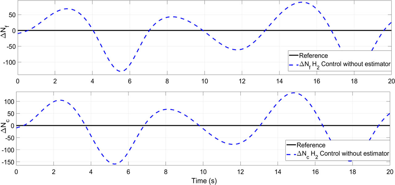
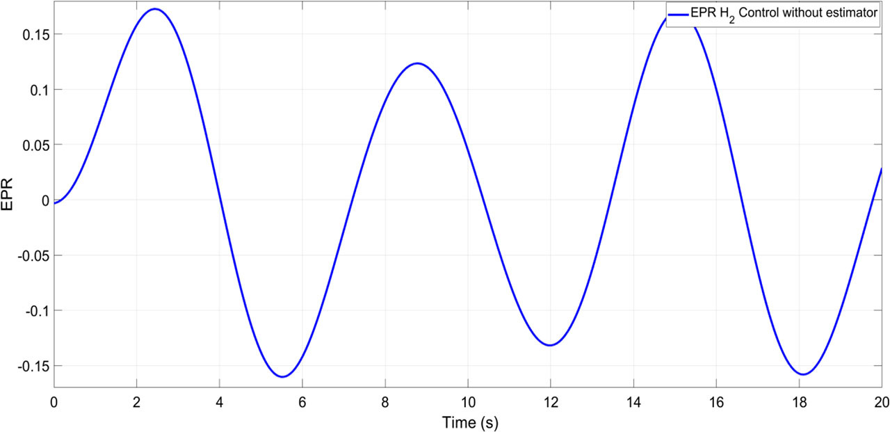
To analyze the effectiveness of the proposed control approach, a standard H₂ controller is designed using the h2syn function in the MATLAB Toolbox. Two scenarios were examined for the standard H₂ control approach. In the first scenario, the GE-90 aero-engine model was simulated using the standard H₂ control without a disturbance estimation. The fan speed and core speed are depicted in Fig. 3, while the EPR increment for the GE-90 aero-engine is shown in Fig. 4. It is evident that the standard H₂ control does not mitigate the disturbance effect. Next, the same model was simulated with the incorporation of the following disturbance observer:

L=−0.0090−0.0043−0.0043−0.0025.

Fig. 3.

The ℋ₂ control responses of the fan and core speed increments without an estimator

Fig. 4.

ℋ₂ control response of the EPR increment without an estimator

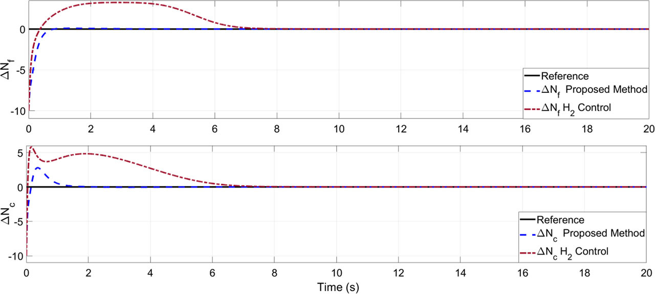
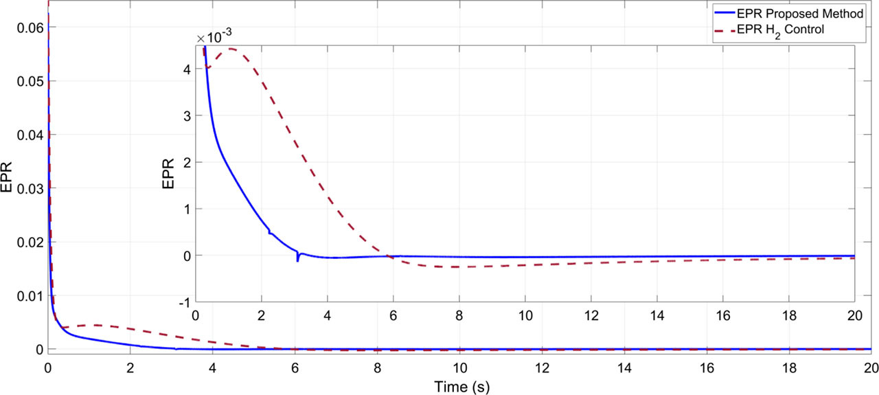
Furthermore, we compare the simulation results of the proposed method and the standard H₂ controller with a disturbance observer. The responses of the fan speed and the core speed are presented in Fig. 5, while the EPR increment of the GE-90 aero-engine is depicted in Fig. 6. In addition, the comparison of the variation between the external disturbance and its estimation is illustrated in Fig. 7. The performance of the disturbance observer, showing that the estimated disturbance closely matches the actual disturbance profile. The system successfully maintains stability and performance, with settling times of EPR = 3.5 s, ΔNc = 1.5s, and ΔNf = 0.8 s using the proposed control structure. In comparison, under the standard H₂ control, the system exhibits settling times of EPR = 20 s, ΔNc = 7 s, and ΔNf = 7 s. This demonstrates the effectiveness of the observer in real-time disturbance estimation. Additionally, the switching function under the dwell-time is displayed in Fig. 8. Incorporating dwell time enhances control performance by reducing energy fluctuations and ensuring system stability. By allowing brief pauses during the switching process, our method mitigates the oscillations typically associated with abrupt transitions, fostering a more stable operational environment. Notably, the time-varying nature of our approach facilitates smoother transitions, avoiding the harsh shifts that can destabilize the system. This smoothness not only improves overall responsiveness but also contributes to a more reliable control strategy, reinforcing the advantages of our proposed method compared to existing techniques. Overall, the simulation results confirm that the proposed anti-disturbance control scheme effectively eliminates the external disturbance given in (31) and stabilizes the nonlinear validation model of the GE-90 aero-engine.

Fig. 5.

The fan and core speed increments

Fig. 6.

EPR increment

5. CONCLUSION

This paper tackles the composite anti-disturbance switched control problem for switched systems. The dwell time approach has been used to analyze the robust stability with ℋ₂-norm performance index using the linear matrix inequalities conditions. The gains of the switched ℋ₂ controller and the gain of the disturbance observer are computed by solving a convex LMI optimization problem. Then, the proposed control scheme is successfully implemented in an aero-engine model. A standard ℋ₂ controller method is used to analyse the efficiency of the proposed control approach. Simulation results validate the effectiveness of the proposed control scheme under the external disturbance. In future works, we will consider the disturbance suppression with input saturation problem in the application of aerospace systems.