
INTRODUCTION
Nowadays, there remains a growing demand for greater accuracy and reliability of the models used for predicting the lifetime of structures working at elevated temperatures. Not only can the absolute lifetime be evaluated, but relative parameters like safety margins also contain important information. They enable the prediction of the remaining time after the first symptoms of damage are noticed.
In order to assess the safety margin, the lifetime of a component working in creep conditions is divided into two stages. The first stage is characterised by the development of internal damage. This stage, called the pre-cracking process, is terminated when the first macroscopically observed damage occurs, this time is denoted by ti. In the second stage, the defects spread to form a single crack or a field of cracks or voids (cf. [1]). This is called post-cracking. The mode of this development depends on the material properties as well as on the geometry of the specimen and the environmental conditions. At the beginning of this stage, the crack develops in a stationary manner. The strain rate is almost constant and the stress distribution around the crack tip follows the crack tip position, i.e. it is constant in time as a function of position relative to the current crack tip. At the end of the process, one can observe the acceleration of the crack growth. In this stage, the length of the crack reaches its critical size, i.e. the final fracture occurs. The total time to failure is denoted by tf. The safety margin is defined by ratio tf/ti.
The first stage can be described by damage mechanics (DM) methods. The second one is the domain of fracture mechanics (FM), but the DM approach can also be involved. The FM methods give a much more relevant solution of the problem of crack growth, but DM allows for a better understanding of the crack propagation process, especially for complex geometrical and material configurations.
In the current work, the stress-based model of damage development originally proposed by Kachanov [2] and then developed by Rabotnov [3] was examined. Its description of the crack growth process in creep conditions was compared with the results of FM analysis. As a basic tool, the finite element method (FEM) was used. The non-local integral method was applied in order to regularise the solution. Many other models of damage development exist, such as the stress-based Murakami-Liu model (e.g. [4]), strain-based models (e.g. [5]), the micromechanical model (e.g. [6]). There are also many methods of numerical solution, like XFEM (e.g. [7]), the eikonal non-local method (e.g. [8]) and gradient methods of regularisation (e.g. [9]). However, they usually require very specialised tools. Additionally some stress-based DM methods, to accurately describe the crack growth process introduce several damage parameters [10,11,12]. This, in turn, requires the identification of many material parameters, which is not straightforward due to the time-consuming nature of damage testing under creep conditions.
The aim of the current paper is to show the capabilities of the application of a relatively simple Kachanov equation in order to solve a given problem. The C(t)-integral, as well as the time to failure were determined for a material with developing damage using the numerical method proposed by the author. Additionally, a nonlocal method already proposed in [13] has been developed using the DM approach, where averaging is performed with a weighting function over an area limited by the interaction radius.
The main goal of the present work is to compare the mentioned methods and their applicability to studying various stages of crack development under creep conditions. This will allow for the establishment of a safety margin, i.e., a parameter that enables the estimation of the lifetime of structural elements based on the observed first signs of damage.
To illustrate the problem, the cracking of a specimen made of 316 stainless steel at a temperature of 550°C was analysed. The 316SS is widely used, e.g. in pressure vessels in nuclear reactors, especially at elevated temperatures where creep and creep-fatigue resistance are of primary importance.
There are numerous items of experimental data available in the literature for this material, both for the tension of initially undamaged specimens and for compact tension (CT) specimens (e.g. [14,15,16,17,18]). The typical operating temperature for pressure vessels made of 316 steel is about 0.4 Tm, where Tm is the melting temperature approximately 1680 K (cf. [19]). Most of the available experimental data pertains to the temperature range of 0.5 to 0.6 Tm, as tests at lower temperatures are more time-consuming. The chosen temperature also falls into this range, as 550°C corresponds to 0.49 Tm.. Therefore, the extension of the obtained results to other temperature ranges should be done with great caution, taking into account the changes in creep and damage mechanisms observed on the corresponding maps (cf. [19,20]).
THE FRACTURE MECHANICS APPROACH
. FM models of creep crack growth (CCG)
The FM approach uses the energy needed for crack development as the main source of information about the process. For a given crack length, it is possible to calculate the critical loading or alternatively the critical crack length for a given loading.
In the first stage of failure development, there is no observable crack, so it is impossible to describe this stage in terms of FM. However, it is possible to correlate this period with FM parameters and determine the time of crack initiation (cf. [21,22]).
In the second stage, FM is mainly used in the case of a single crack. If the stress field around the crack tip is known, the J-integral or its creep equivalents C* or C(t) can be calculated. The definition of the C* contour integral is similar to the J-integral but strains and displacements are replaced by their rates (cf. [22,23]):
whereWhen the stationary creep does not occur, the stress field around the crack tip can be described by the C(t) parameter [24]:
This integral is not path independent, it has to be evaluated near the crack tip. For a large t, when creep becomes stationary, C(t) approaches the C*-integral, for any t: C(t) > C*. It was shown that in stationary creep conditions, the C*-integral can be correlated with the crack growth rate (cf. e.g. [21,25,26]).
. FM estimation of lifetime
The time for crack initiation ti is not directly described by FM models. There are some estimations, and the proposition of Tan, Celard et al. [21] is applied in the current work. They defined a lower and upper approximation. The first formula uses the typical relation between the C* parameter and crack growth rate:
where a is the current crack length, and D and φ are material parameters. To calculate the time ti, the initial crack increment da is assumed. This increment is assessed as the minimum crack length which can be measured. This approach gives the lower approximation of the crack initiation time:The upper approximation tiU is achieved under assumption that the initial crack growth rate is (n+1) times smaller than the rate in a stationary state, where n is creep index in the Norton creep eq. (8):
The comparison of the results of experiments for different steels with the approximations defined above indicated that the crack initiation times fall within the expected range. The lower approximation was closer to the experimental results in most of the examined cases (cf. [21]).
The next step in the determination of the safety margin is the estimation of the crack growth time period tf-ti. This is usually determined though the integration of eq. (3), starting from the initial crack length ai=da up to the final crack length af which is equal to the total width of the element (cf. [27]). To perform this integration, the relationship between the value of the C* parameter and the current crack length has to be established. This relationship can either be obtained analytically (cf. [22]) or numerically. This approach is limited by the assumption that the crack grows in a stationary environment, i.e. the stress distribution in the vicinity of the crack tip is described by stationary creep equations. This is possible only when the rate of stress redistribution is faster than the rate of crack growth. If this assumption is not satisfied, the C*-integral cannot be used and instead, other parameters, specific to the transition creep period, like C(t) or Ct, can be applied (cf. [28]).
The material parameters D, φ (eq. (3)) can be found experimentally or determined by some analytical formulas (see [22]). There is also an approximate solution which describes the creep crack growth quite well for most of the cases (cf. [5]):
whileTHE DAMAGE MECHANICS APPROACH
. Uniaxial tension creep damage model
All of the formulas of FM are valid only in situations where an initial crack exists. Parameters like C*, C(t) are undefined for uncracked specimens. There is no such limitation in the case of damage mechanics models. The damage develops in material that is initially undamaged, which leads to the initiation of a microcrack. Therefore, DM can be used for determination of the time ti. It is also possible to model the flaws or microcrack systems in original material by setting an appropriate initial damage field.
When the crack starts to develop, the application of DM is more troublesome. However, attempts to describe the crack development by growth of the damage field up to its critical value and further development are often made (cf. e.g. [5,25,29,30,31]).
This approach, known as the local approach to fracture (LAF) encounters a series of problems [32]. Applications of continuous equations in the solving of DM problems (named continuous damage mechanics [33]) are limited by the size of the smallest element in which system variables can be considered continuous, called representative volume element (RVE). The requirements for RVE are contradictory. RVE should be large enough to contain the representative number of defects and sufficiently small that the variations of stress and strain values are relatively small. These requirements can be more or less satisfied for a problem with undamaged or randomly distributed damage to the material (cf. [34]). The damage distribution is usually corelated with the microstructure of the material and the size of RVE is then adopted to the characteristic dimensions of this microstructure.
In the original Kachanov model [2] and in its successors (e.g. [4,18,35]), the development of damage is dependent upon the stress state. There are also strain-based damage models (e.g. [15,36,37]) in which the critical value of the damage parameter is achieved when the ductility of material is exhausted. The current work is mainly based on the Kachanov proposition of creep damage development. Additionally, it is assumed that the creep strains are associated with damage (cf. [3]). The uniaxial constitutive equations are as follows:
where σ is uniaxial stress,. Influence of stress triaxiality
The equations of the development of creep damage are fitted to experimental results in the uniaxial tension creep test. While the triaxial stress state is achieved in the vicinity of the crack tip (cf. e.g. [15,18,35,38]). Hayhurst, who analysed the growth of damage in the multiaxial state, assumed that effective stress σeff is responsible for damage development and it takes the form [39]:
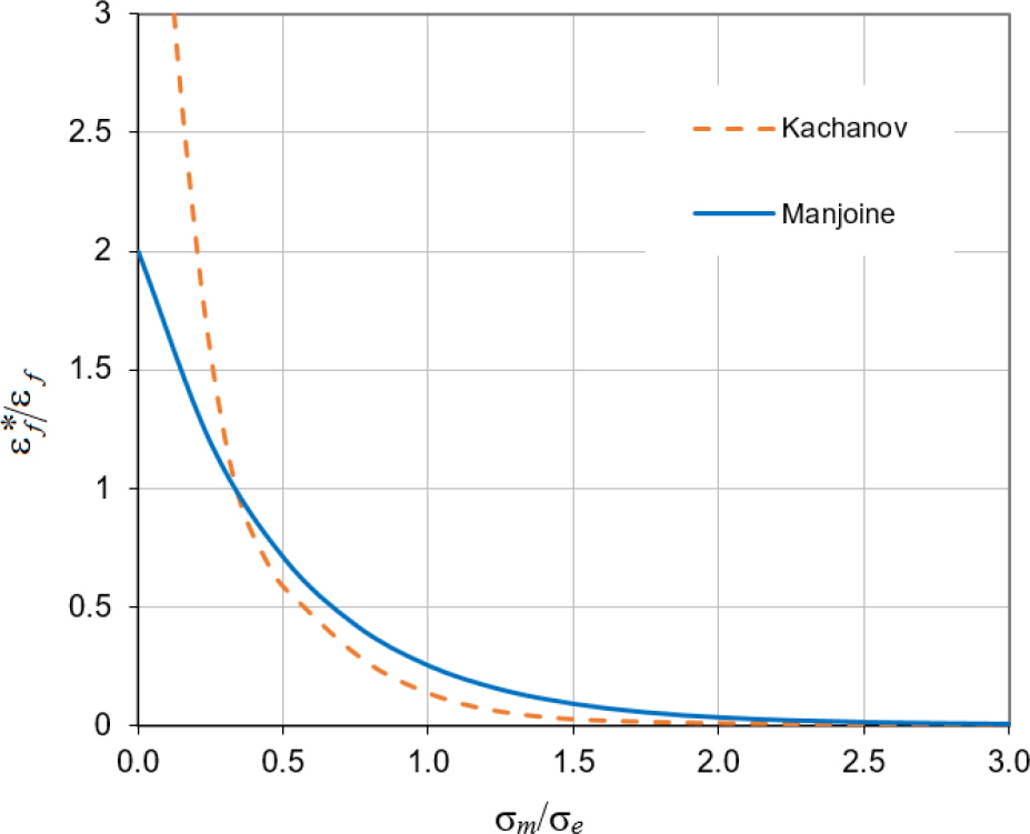
where α, β, γ are material parameters, σmax is maximum principal stress, σm is mean stress and σe is Huber-von Mises-Hencky equivalent stress. The influence of σm is negligible for metallic materials as it is responsible for the volumetric growth of voids and creep deformation is regarded as incompressible. Then eq. (10) reduces to: and the effect of stress triaxiality is solely described by parameter α. This approach is widely used in many stress-based damage models (cf. e.g. [4,25,35]).In models where the damage parameter is based on strain, the ductility is described by the Manjoine equation (cf. e.g. [4,15,40]):
Here, the ductility is a function of the triaxiality coefficient defined as ratio σm/σe. In the vicinity of the crack tip, the value of this coefficient is large, so the strain at failure is small (cf. [18]). In Fig. 1 it can be seen that the strain at failure calculated from the Kachanov model (eqs. (7–8, 11)) is close to the Manjoine model in this range.
. Non-local damage model
The main problem in the application of continuous DM equations is strong localised damage and strain occurring in the numerical solution of crack problems. It results in the spurious mesh dependence of the solution (cf. [41]).
There are many possibilities to prevent excessive damage localisation, such as the mesh-dependent softening modulus, the limitation of mesh size, artificial viscosity, the Cosserat continuum, the gradient method and the non-local integral method (see [42] for review). The non-local damage theory seems to be one of the most popular theories. The idea is that the constitutive equation contains not only local values but also some non-local parameters obtained by averaging the chosen value in a particular volume. The motivation for the use of non-local theory is the observation that the growth of the crack does not depend on the state at a given point but on energy release in its vicinity (cf. [43]). This method is also used in the current work.
The definition of the non-local value of the state variable is:
where V(x) is the neighbourhood of point x, w(x,r) is the weighted function, and is the characteristic volume (cf. [44]).The value of weighted function depends on the relative position of points x and r. The most popular version of it is Gaussian distribution:
where d(x,r) is the distance between points x, r, and d* is the characteristic length. The characteristic length becomes a new method parameter. Usually, it is a material parameter, depended on the internal structure of the material. For crystalline materials, it has to be associated with grain size (cf. e.g. [13,45]). According to some authors, it is not a pure material parameter as it is also dependent on the used solution method (cf. e.g. [46,47]).Theoretically, the size of the neighbourhood V(x) can be unlimited, but for practical reason, it is limited to some extension of characteristic length. The smallest distance between points x and r, at which the weighted function vanishes or becomes negligible, is called the non-local interaction radius (cf. [43]). There are also methods for which the interaction radius is exactly equal to the characteristic length (e.g. grid method [13,48]).
CREEP CRACK GROWTH SIMULATION OF CT SPECIMEN
. Experiment description
The analysis was performed for a compact tension (CT) specimen made of 316 stainless steel creeping at a temperature of 550°C. Its results were compared with experimental data [18]. The dimensions of the specimen are presented in Fig. 2 and Table 1. The CT specimen was prepared according to the standard procedure given in ASTM E-399. The loading was 19,620 N which gives a time to rupture of about 40 200 hours at a temperature of 550°C. The reference stress level calculated according to [18] is 164 MPa. The fracture toughness of 316 stainless steel is about 240 MPam0.5 at room temperature and it is reduced by about half at 550°C (cf. [49]). A similar reduction can also be found in [50].
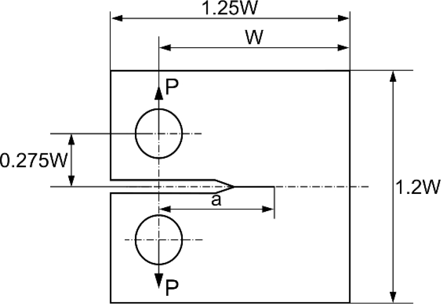
Tab. 1.
Parameters of CT test [18]
| T [°C] | W [cm] | B (width) [cm] | a [cm] | P [kN] | tf [h] |
|---|---|---|---|---|---|
| 550 | 50 | 25 | 16.67 | 19.620 | 40 200 |
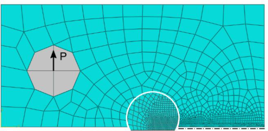
The specimen was modelled in the Abaqus Finite Element system in plane strain. Due to symmetry, only half of each specimen was modelled. The example of the mesh with symmetric boundary conditions is presented in Fig. 3.
The material parameters were determined on the basis of uniaxial creep tests at a temperature of 550°C (cf. [14,18]). They are as follows: elasticity modulus E=169617 MPa, Poisson ratio ν=0.3, creep deformation parameters: B=6.561E-24 (MPa)-n h-1, n=7.778, damage development parameters: A=3.983E–23 (MPa)-mh-1, m=7.622. Additionally, the dependency of instantaneous strain ε0 was modelled on the basis of plastic deformation and primary creep.
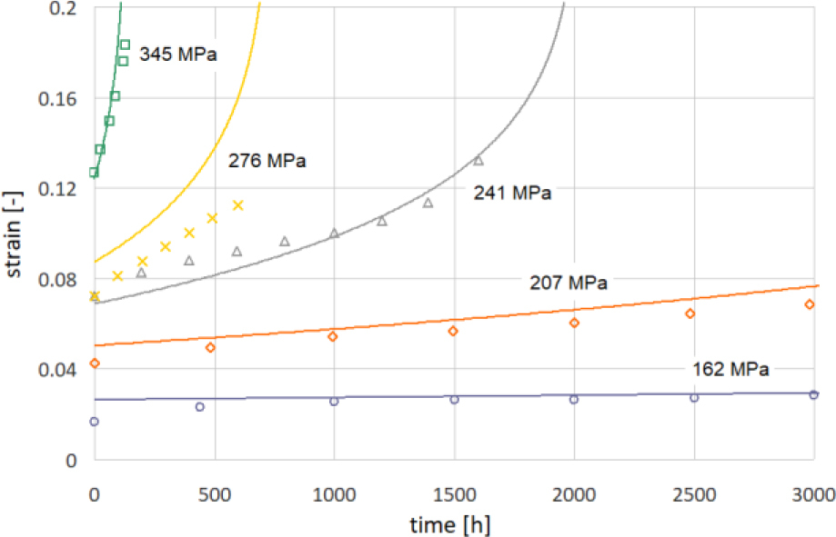
It can be observed in Fig. 4 that the Kachanov eqs. (7–8) assure a good approximation of strains in the secondary creep period but exceed the experimental values for tertiary creep. It affects the strain at failure but does not change the time to failure which is the main target of the analysis.
Fig. 4.
Comparison of results of the Kachanov model with chosen experimental points of uniaxial tension creep of 316 steel at a temperature of 550°C [14]
To model the influence of stress triaxiality, equation (11) is used. Parameter α was determined by Hayhurst et al. [14] in the notched bar tension experiments and the value of α=0.75 was used in the current paper.
. FM crack growth simulation for stationary creep
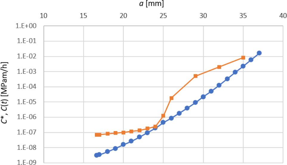
In order to simulate the crack growth, the C*-integral was used. The dependency of C* on crack length was found using finite element analysis. The built-in procedure of Abaqus system (cf. [51]) was used for the determination of the C(t) parameter and then the limit value of it in the stationary state was established as the C* value. The Norton creep model – eq. (8) – without damage development (ω=0) was used as a constitutive equation. The results of this analysis are presented in Fig. 5 (blue line).
Fig. 5.
C*-integral for stationary creep (blue circles), and C(t) for a model with damage (orange squares) as a function of crack length
Next, the value of ti (crack initiation) was established. Eqs. (4–5) require knowledge of material parameters D and φ. The approximate values of these parameters are defined in eq. (6). The index φ is equal to 0.85 and the value of parameter D is equal to 692.3, assuming a plane strain state and ductility of εf=0.13 (cf. [14]). Using these values, the lower estimation of initiation time is 12.6E3 h and the upper estimation is 110.8E3 h for da=0.5mm. The upper estimation is much larger than the experimental value of the time of final failure; therefore, the lower estimation was chosen for future analysis. Such an approach also corresponds to the results presented in [22].
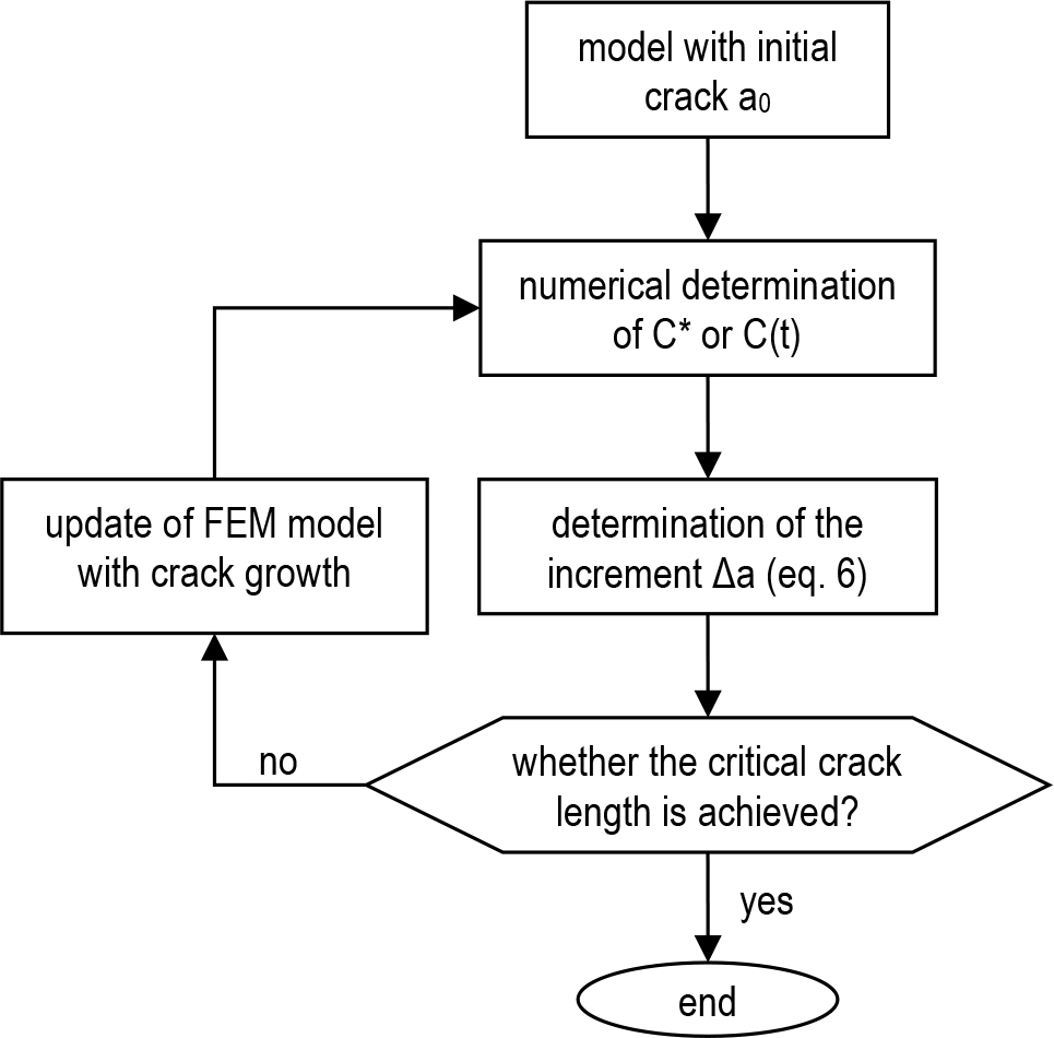
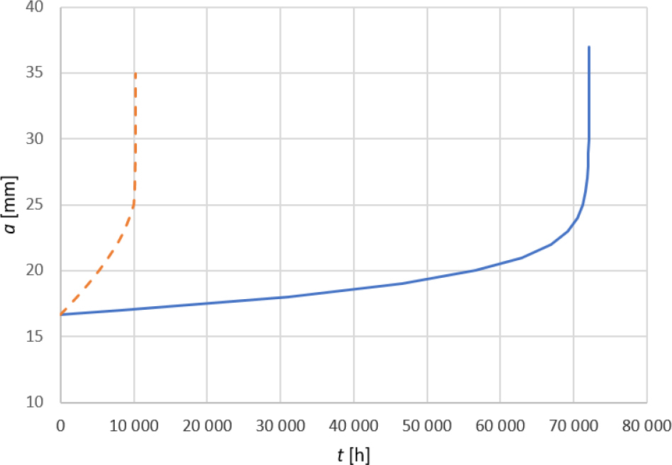
The simulation of crack growth was obtained by the integration of eq. (6). The simplified flowchart of the applied procedure is presented in Fig. 6. The result is presented in Fig. 7 – solid blue line. The time to failure tf obtained in this method (sum of the initiation time and crack growth time) is 84.7E3 h, which is two times greater than the experimental value. The safety margin according to this method is tf/ti=84.7/12.6=6.7.
. FM crack growth simulation for the creep damage model
The method described above can be applied when in the vicinity of the crack tip, the stress distribution reflects the stationary state. This is the case when stress redistribution is faster than crack growth. The duration of stress redistribution can be calculated from the formula (cf. [1]):
where the J-integral describes the initial plastic distribution. This time for the examined case is equal to 124E3 h, so it is much greater than the expected time of crack growth. This is the reason that the stationary creep model does not describe the case well.The second model considers the damage field developing prior to the crack formation. As a consequence, the crack growth is faster and the time to failure shorter. The full set of eqs. (7–9) is used in this case. When the damage parameter reaches its critical value (0.99) at an integration point, this point is marked as damaged and excluded from the problem domain. The cluster of such points forms a crack or a void ahead of the crack tip.
In these conditions, it is impossible to reach the stationary distribution and determine the C* parameter. The C(t) defined by eq. (2) can be used instead (cf. [1,22]). There are not many works using this approach (cf. [52,53]); therefore, a custom procedure based on the scheme presented in Fig. 6 was used. The value of C(t) integral is determined at the moment just before the damage parameter reaches its critical value. The obtained results for different crack lengths are presented in Fig. 5 (orange line). These values are greater than the corresponding C* values, but for small crack lengths, the increment of C(t) is smaller, which generates a more stable rate of crack growth of order 1E-3 mm/h. The change of dependency function can be observed when the crack length achieves about 25 mm, which can be considered as the critical length.
The parameters of eq. (3) are the same as in the previous model. The index φ in the damaged environment is often equal to (cf. [54]):
However, in the examined case, this expression gives a value very close to the approximate value given by eq. (6), which was finally chosen (0.868 vs. 0.85).
The curve of crack growth obtained on the basis of the above assumptions is presented in Fig. 7 (dashed orange line). The time of crack growth up to failure is 10.2E3 h, and total time including the initiation time is 22.8E3 h. This value is about two times smaller than the experimental time and the safety margin obtained in this model is tf/ti=1.8. It is much smaller than predicted by the previous analysis and can be used as its lower approximation.
. DM local model
In the next step, the local Kachanov model described by eqs. (7–9) was used. The material parameters were listed in Section 4.1. As the solution is strongly mesh-dependent, the simulations were performed for four meshes with a minimum mesh size from 0.5 to 0.05 mm. The times ti and tf obtained in these simulations are presented in Fig. 8. Despite the large spread of results, it can be noticed that the safety margin tf/ti is more repetitive and it falls between 2.0 and 2.6, except for one case (a very rare mesh). The lower bound of this range can be used as an appropriate approximation of the ratio tf/ti.
Fig. 8.
Crack initiation time ti and the time to failure tf as a function of minimum mesh size for local and non-local damage models
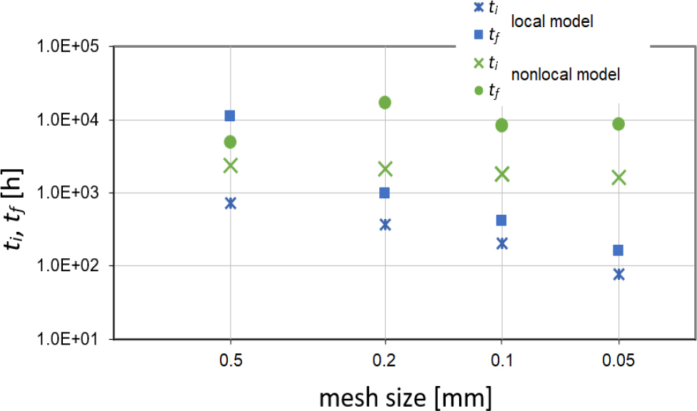
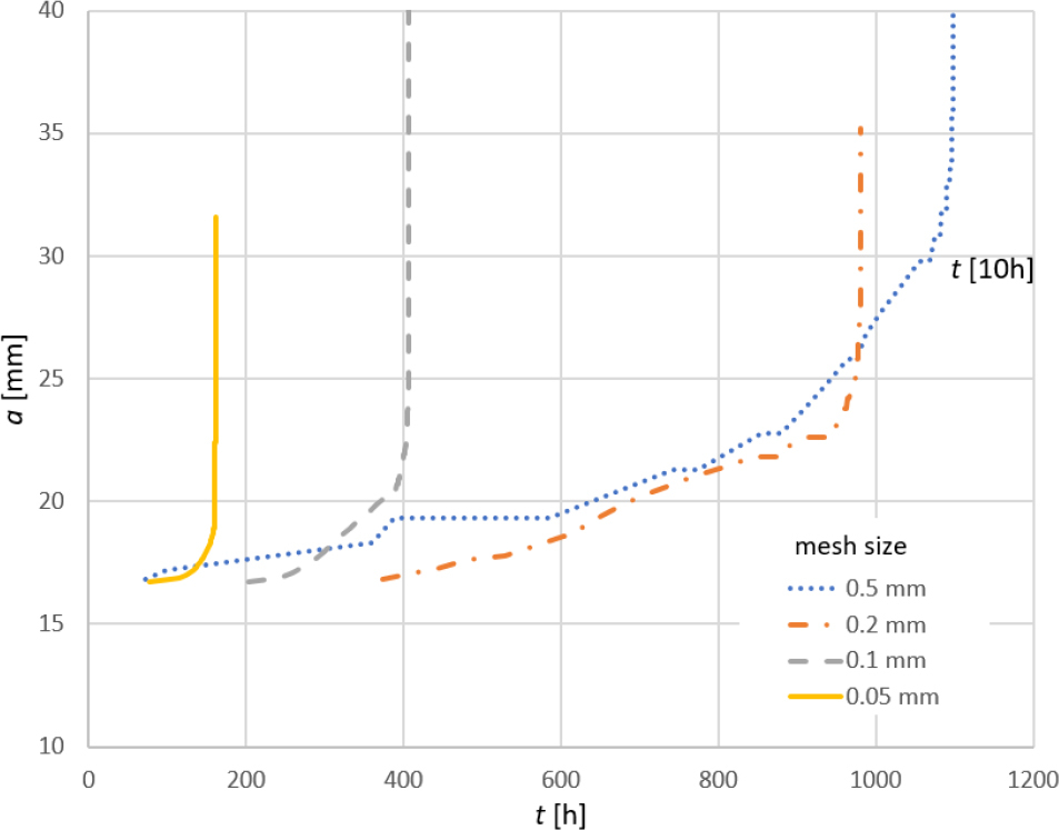
For the examined model, the value of time to failure parameter tf is within the range of 160 h to 11E3 h, indicating a very large spread. All calculated values are smaller than the experimental value. The crack was developing in a plane of initial crack, as it was expected. Its growth rate is initially stationary at the level of 2E-2 mm/h (see Fig. 9). From Fig. 9, the approximate value of critical crack length can also be determined. Its value depends on the mesh density and varies from 20 to 32 mm.
. DM non-local model
In the non-local model, the state of point depends not only on the previous state of the point but also on the state of neighbouring points. This causes the time to rupture of the cracked specimen to be greater than that obtained in the local method as the factors influencing the damage growth are volume averaged.
Different state variables can be averaged (see [43] for review). The most popular formulation assumes that the damage variable depends on averaged strains (cf. e.g. [45,55,56,57,58]). In the current work, damage development is a function of stress and the damage increment was chosen as the averaged parameter. Such an approach was proposed by Chaboche (cf. e.g. [13,44,59]). First, the local damage increment is calculated:
In the next stage, the equation of damage growth is formulated in terms of the average value of damage growth. It is calculated with use a formula derived from eq. (13):
where the weighted function w(x,r) and the volume Vr are determined according to formulas (14-15). In these equations, the characteristic length parameter d* plays the key role. In the present work, it is assumed to be equal to parameter da used in FM model, i.e. 0.5 mm. The volume V(x) was bounded and the interaction radius was assumed to be equal to 3d*.The application of the non-local method enabled the obtaining of the time to crack initiation ti which is much less dependent on mesh size than in the local model. Its dispersion was from 1.6E3 to 2.3E3 h. The value of the tf parameter was much more scattered, from 5E3 to 17E3 h, but it was still more stable than in case of the local method. According to the performed simulations, the estimation of the safety margin is between 2 and 4, which is slightly more than that obtained from previous methods.
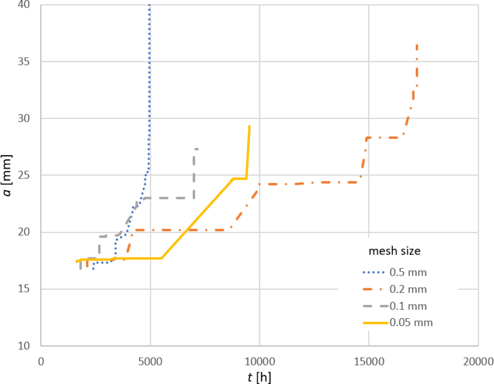
By comparison of the growth curves for different mesh sizes, one can notice that they are close to each other in the initial period. Thus, the goal of the application of the non-local method was achieved. Further development of the crack follows by step increments and the differences between individual solutions are observed. This indicates that an unambiguous solution cannot be achieved for time tf using the presented method. Despite it can be noticed that all solutions give a common starting point for fast crack development, this point can be approximated as 25 mm of crack length. This result aligns very well with the previously obtained solution using FM in the damaged environment.
SUMMARY
The presented solutions to the crack growth problem under creep conditions did not yield fully satisfactory results. The obtained times exhibit significant variability. In the case of the FM methods, the time to crack initiation depends primarily on the parameter da. Its role is similar to the mesh size in the finite element method (FEM) or the characteristic length for non-local methods. The shortest time to failure was achieved in the local model, but it strongly depends on the mesh size. The non-local method provides a prediction of crack initiation time independent of mesh size, thus achieving the intended goal. However, this approximation is significantly smaller than the lower bound estimate obtained using the method proposed by Tan, Celard et al. [21]. Obtaining larger times to failure in simulations is possible by adjusting the parameter α (see discussion below).
A significant spread of results was also obtained for the time to failure. FM-based methods yield longer times than the empirical ones, while DM-based methods yield shorter times. The longest time of crack growth was determined using the C* parameter. However, this method assumes the stationary stress distribution in the vicinity of the crack tip, which is unattainable. Other methods based on damage mechanics yield more realistic results, although these are lower than the experimental values. Nevertheless, they are on the safe side, making them suitable for estimating time to failure in situations where initial signs of damage are observed.
Despite the discrepancy in specific times, the comparison of safety margin estimates tf/ti presented in this paper yields very similar results. Especially, the local DM method provides a relatively constant value of safety margin, meaning that the time to rupture is proportional to the time of initiation, regardless of the element size. On the other hand, the non-local method exhibits a larger spread in safety margin due to the variability in time to rupture, while maintaining a constant initiation time. The non-local method also clearly indicates a critical crack length, which is the value at which a rapid increase in crack growth velocity occurs. Its value is also consistent with the result obtained using the C(t) integral.
The key problem of these predictions is also the availability and reliability of material parameters. There is large dispersion of material data for examined steel (cf. [16]). Additionally, they are mainly determined in uniaxial creep tension experiments, but are used in situations in which the multiaxial stress state dominates. Only the parameters of eq. (10) are responsible for this behaviour, so their proper determination is crucial. To solve this problem, Hyde proposed calibration of the value of parameter α by fitting the time to rapture in the CT experiment [35]. They obtained value α=0.48 for similar material at a temperature of 600°C. The smaller value of parameter α gives larger time to failure, so closer to experimental value. However, the application of this approach raises many doubts. It should be used only when the numerical simulations produce unambiguous results. Since this is not the case here, applying this method is not possible.
The solutions obtained by the author enables drawing the conclusion that the most reliable results are obtained from the C(t) method and the non-local DM model, which are very close to each other. These methods, despite some limitations, are relatively simple and they can therefore be used in the estimation of lifetimes to fracture and safety margins for structures undergoing cracking in creep conditions.