INTRODUCTION
Numerical simulations has become an important tool for analysing transport phenomena occurring in many complicated devices, including heat exchangers. This method allow researchers to estimate flow behaviour and thermal performance without relying only on experimental investigations. Preparing and operating experimental test stands for such studies is often associated with high costs and spatial challenges. The heat exchangers are designed to transfer heat between fluids of unequal temperatures moving through internal flow passages. The present study investigates a shell-and-tube heat exchanger with semicircular tubes. To enhance the intensity of heat transfer, the tubes may be equipped with fins. They are plates manufactured from materials characterised by high thermal conductivity. Increasing the effective heat exchange surface improves the thermal characteristics of the exchanger. However, the additional elements on the flow path may simultaneously increase flow resistance and consequently influence the overall efficiency of the system.
The literature offers numerous studies on methods to enhance the heat transfer rate. Advancements in material science and chemistry offer new materials in heat exchangers design [1, 2] or the novel working fluids [3–6]. The geometric modifications, such as changing the shapes of tubes or fins, are a common method to achieve this goal. Circular tube heat exchangers have been most extensively examined in various configurations, due to their application popularity. Evaluations of their performance were conducted in a wide range of Reynolds numbers, both experimentally and numerically [7–9]. The scientists further investigated the effect of changing the shape of tubes to a cam [10] or wing [11]. Various, not fully symmetrical shapes, have opened up the field for investigating favourable angles for heat transfer rate. The extended surface elements are not limited to only rectangular plates. There appeared articles applying transverse or longitudinal, wavy, spiral, serrated, and perforated [12], elongated hexagonal, segmented [13] or flexible fins [14].
The plain semicircular tubes have been studied in literature describing their thermal performance and flow resistance as single tubes [15–17], or in arrays [18, 19]. There was also a determination of thermal and hydraulic performance study conducted over a single tube with a longitudinal fin on one or both sides [20]. However, the arrays with longitudinal fins have not been investigated in detail. This relevantly new topic was formerly discussed by Afifi et al. [21] and Szydłowski and Gutkowski [22] with the use of numerical simulations. To the authors’ knowledge, there were no previous studies concerning semicircular longitudinally tubes with wavy fins in a staggered arrangement.
The application of the wavy fins is popular in circular or elliptical tube heat exchangers. Qiu-Wang Wang et al. [23] have assessed numerically the thermal-hydraulic performance of single, longitudinally finned circular tubes in a range of Reynolds numbers from 904 to 4,520. The authors prepared three geometries: plain, interrupted wavy fin and sinusoidal wavy fin. Wavy fins increased heat transfer by up to 90% while also raising the pressure drop by more than four times at most. Elliptical and circular tube heat exchangers were examined by Y. B. Tao et al. [24] at Re = 500-4,000. Elliptical tubes with transverse wavy fins provide 30% higher heat transfer and a 10% increase in friction factor compared to circular tubes. Similar studies were conducted for a heat exchanger with six-tube-bundle by W.-X. Chu et al. [25] for inlet velocities ranging from 1 to 6 m/s, corresponding to Reynolds numbers of approximately 2,300–14,500. Their results demonstrated that the spacing between sinusoidal wavy fins significantly affects both the pressure drop and heat transfer performance. For circular tubes, the smallest studied fin spacing reduced the pressure drop by approximately 10%, whereas the largest spacing increased it by about 10%, in comparison to the oval tubes. Increasing the fin spacing enhanced the heat transfer rate by up to 20% for circular tubes and 25% for the oval ones. Transverse wavy fins of different amplitude coefficients in the range of Re=1,000-5,500 were under the scope of Junqi Dong et al. [26]. The results indicate that the waviness amplitude significantly affects heat transfer and pressure drop, whereas the fin profile type has a minor influence. A larger waviness amplitude increases heat transfer, while a smaller amplitude yields a higher j/f (Colburn to friction factor) ratio.
The topic of increasing heat transfer rate is common and has already been studied for a long time. More and more ideas for the tube and fin shapes are appearing in the literature. Although wavy fins have been investigated before, this article presents the unique results for a longitudinally wavy-finned semicircular heat exchanger with a bundle of eight tubes. It extends the current research on wavy fins by simultaneously: (1) considering the relatively unexplored semicircular tubes instead of circular or elliptical ones, (2) applying them in the longitudinal direction for a tube bundle, and (3) investigating their thermal-hydraulic performance over a wide range of Reynolds number. Comparison of different fin lengths and the Reynolds number will allow the reader to find the proper combination for the desired application. The simulations were conducted for five geometrical configurations (from plain to fully joined fins), and each configuration was subjected to ten different inlet velocities referred to the Reynolds number (from 1,000 to 10,000).
NUMERICAL MODEL
The aim of the present study is to create a model focused solely on thermal performance intensification caused by the modification of tubes in a heat exchanger. The flow and heat transfer were modelled for the repeating, smaller array of tubes of a larger tube bundle, far from the heat exchanger casing or headers. Parameter values were gathered to present an indication of the potential improvement level for long-term, stable operation. Thus, the flow of air through the heat exchanger was simplified to two dimensions and a steady state. The modelling software was ANSYS Fluent 2024 R2. The air was treated as an incompressible and Newtonian fluid with constant physical properties corresponding to 300 K. The flow was recognised as turbulent due to the geometry and the Reynolds number range. Calculations in such cases are performed based on the equations of flow continuity, mass and momentum conservation, and turbulence, depending on the applied turbulence model. The boundary conditions have been similar to the popular methods in heat exchangers’ simulations. First, a maximum velocity was calculated according to Eq. (1). Such a velocity may occur between the tubes of the same row or between the neighbouring tubes from different rows. Knowing where the distance is the smallest, the calculation is performed. In this work, the maximum velocity vmax was reached between the tubes of the same row.

where ReD, max – largest reached Reynolds number based on the tube diameter [-], μ – dynamic viscosity [kg/(m·s)], ρ – fluid density [kg/m3], D – tube diameter [m].
The inlet velocity vin was found through applying the continuity formula with case-specific geometrical relations, deriving Eq. (2). This velocity was later applied as the inlet boundary condition.

where PT – transverse axial pitch [m].
Thermal performance was assessed through the average Nusselt number N̅u̅D, that was calculated with Eq. (3) for every simulated case. The formula requires prior finding a logarithmic temperature difference ∆Tl through Eq. (4) and the average heat transfer coefficient h̅ through Eq. (5). The surfaces in contact with the fluid had a total area per-unit-span (A), whose value was equal to 1 m.
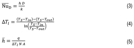
where k – thermal conductivity of air [W/(m·K)], TS – surface temperature [K], Tin – air temperature at inlet [K], Tout – air temperature at outlet [K], q – heat transfer rate per-unit-span [W/m], N – number of rows [-].
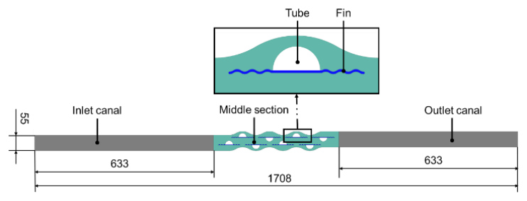
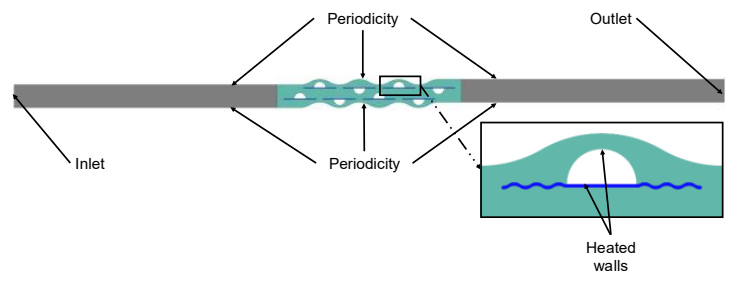
All geometries used in the simulations were prepared in 2D to limit the required computational power. This simplification has been effectively used in previous scientific studies [20–22], with their authors confirming the method’s validity. The designs were divided into three or four sections, depending on the case. All elements are shown in Fig. 1. Two long canals in the vicinity of the inlet and outlet (marked in grey) were meant to stabilise the flow. The tubes (white) and the fins (blue) were in the middle section (green), where the main investigated phenomena occurred. In the case of plain tubes, the fins were not present. The tube diameter was 27.5 mm, and they were spaced horizontally by around 95 mm and vertically by 46 mm. The staggered formation was selected to bring more favourable heat transfer results. Spacing between odd- and even-tube rows was half of the distance between the in-line tubes. The fin amplitude was equal to 2.75 mm, and the thickness was half of it. The diameter of the “waves” was constant, equal to 7.653 mm. The length of the fins was increased from 0 (plain tube) incrementally, every time by one length of the wave, up until the single fins were long enough to join with each other and create a single continuous fin.
A mesh independence study was conducted for the “plain” and “3-wave” cases of semicircular tubes for the highest inlet velocity. The graphs presenting the absolute and relative changes in average Nusselt number for mesh sizes from coarse to fine are shown in Fig. 2. The relative change below 0.3% was approved for the current study. It was observed at an increase to 547,732 elements for the plain tubes and to 587,348 elements for the wavy finned tubes. Thus, the mesh setting delivering the aforementioned values was chosen for all models. The higher number of elements in the finned case is caused by the inflation layer spread over a longer distance. For every case, the mesh metrics were found, and their least favourable average values are gathered in Table 1. The values of y+ for every case at the highest velocity inlet were below two, with the values above one appearing only at a few points on the edge of the fin.
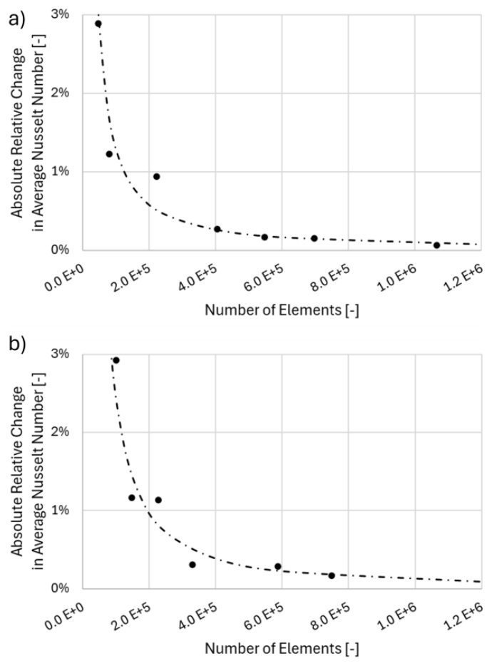
Fig. 2. Mesh independence study comparing the obtained average Nusselt number for the a) “plain” and b) “3-wave” cases
Tab. 1. Average mesh metrics for every geometrical case
| Average of: | PLAIN | FINNED |
|---|---|---|
| Element quality | 0.95 | 0.89 |
| Skewness | 0.08 | 0.11 |
| Aspect ratio | 1.31 | 1.69 |
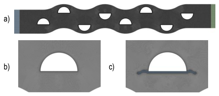
A representation of the selected mesh is shown in Fig. 3 for the whole geometry a) and zoomed at a tube for both the plain b) and finned c) case.
The boundary conditions were set in ANSYS Fluent for two-dimensional geometries, in a steady state with a pressure-based solver with double precision option selected. At the outside edges of the domain a periodic boundary condition was set. Aluminium with thermal conductivity changed to 240 W/(m·K) was chosen as the material for tubes and fins. Fluid domains were filled with air of its constant characteristics at 300 K. A temperature of 400 K was chosen as the thermal condition for all tube-heated walls. The velocity condition was specified at the inlet to refer to Re = 1,000 to 10,000, which meant values of 0.433 m/s to 4.33 m/s. The pressure outlet was set with a gauge pressure equal to 0 Pa. The boundary conditions are presented in Fig. 4. The turbulence model was selected according to a comparison of similar geometrical configurations for plain semicircular tubes [22]. This comparison was made in reference to Zukauskas’s [7] experimental results, and it shows the best compliance for Transition k-kl-ω. Thus, the three-equation model was also chosen for this investigation. Residuals were set to 1·10-7 for energy, 1·10-5 for continuity, x- and y-velocity, kl, kt and omega. Additionally, the behaviour of the residual curves has been observed to confirm their convergence. The pseudo time explicit relaxation factors were left as 0.5 for pressure and momentum, 1 for density, body forces and turbulent viscosity, and 0.75 for the energies and specific dissipation rate. The selected scheme was Coupled with spatial discretisation as Second Order Upwind for most elements (momentum, turbulent and laminar kinetic energy, specific dissipation rate, and energy), with pressure as Second Order and gradient as Least Squares Cell Based. Other settings in the software remained unchanged.
MODEL LIMITATIONS
The computational model represents a simplified version of the full heat-exchanger geometry, and its limitations should be considered when interpreting the results. Beyond the influence of turbulence-model selection and mesh resolution, several additional limitations apply. The investigated model omits the casing and inlet, outlet manifolds, being present in a real full heat exchanger geometry. In reality, these regions may generate turbulence and strong flow disturbances that could alter the measured parameters. Furthermore, the simulation was carried out in two dimensions, which restricts the development of secondary flows and three-dimensional vortex structures, particularly those forming behind the tubes and fins. Because the analysis was performed under steady-state conditions, transient phenomena, such as start-up behaviour, periodic instabilities, vortex shedding, or fluctuating flow separation, are not captured. The visualised fields, therefore, represent time-averaged flow behaviour corresponding to a heat exchanger operating under stabilised conditions. The inlet section was intentionally extended to ensure a uniform velocity profile upstream of the heat exchanger tube bundle. Such idealised inflow conditions may not occur in practical applications. Similarly, the assumption of constant tube temperature does not reflect real operation, even in systems designed to maintain a fixed wall temperature, such as condensers. In applications such as condensers or evaporators, where the wall temperature can be considered approximately uniform, the adopted boundary condition closely reflects real operating conditions. In other configurations, variable wall temperature or conjugate heat transfer effects could alter the local heat transfer coefficient distribution, particularly near the tube-fin junction. However, since the primary objective of this study is a comparative assessment of fin geometries under identical thermal boundary conditions, the constant wall temperature assumption does not affect the relative conclusions drawn.
The working fluid was modelled as air, treated as Newtonian, incompressible, and ideal, with constant physical properties except for density, which varied only with temperature. At the simulated velocities, these simplifications are not expected to significantly affect the overall results. Variations in the thermal conductivity of the aluminium components were also neglected, as convection dominates the heat-transfer process in this configuration.
DISCUSSION OF THE RESULTS
The results were compared within the following measures: velocity and temperature distribution, pressure with friction factor, heat transfer rate and local Heat Transfer Coefficient, and outlet temperature. Some measures were normalised to allow the authors to present the outcomes comparatively for all cases.
Velocity
A graphical representation of the fluid flow was shown with the contours and streamlines of normalised velocity (vnor) calculated with the Eq. (6):

Three configurations of a heat exchanger with semicircular tubes are shown: plain (Fig. 5), finned with the length of three waves (Fig. 6) and finned in a joined manner (Fig. 7). The maximal velocities occurred in every case in the regions between the tubes in a perpendicular direction to the flow. In all cases at Re = 1,000, the stagnation regions were growing within the next rows, while at Re = 10,000, they were getting smaller in those locations. The tubes with fins experience higher normalised velocity than the “plain” case, with its maximum for the “joined” case.
Comparison of the results for the highest and lowest achievable value of Reynolds number indicates that the normalised velocity decreases with an increase in the inlet velocity, but the intensification points remain in the same locations.
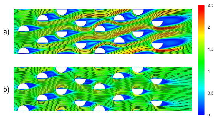
Fig. 5. Streamlines and normalised contours of velocity in plain tube configuration for: a) Re = 1,000, b) Re = 10,000
The addition of fins results in the formation of stagnation regions already upstream of the tube, aligned with the flow direction. The tip of the fin becomes the first element to get in contact with the fluid flow. In the case of tubes with two wavelengths of the fin (Fig. 6), the flow is disturbed earlier and thus, the stagnation zones appear at the connection point between the tube and fin. Moreover, there is no clearly visible recirculation downstream of the tube. The recirculation also takes place there, but it is at a much lower velocity.
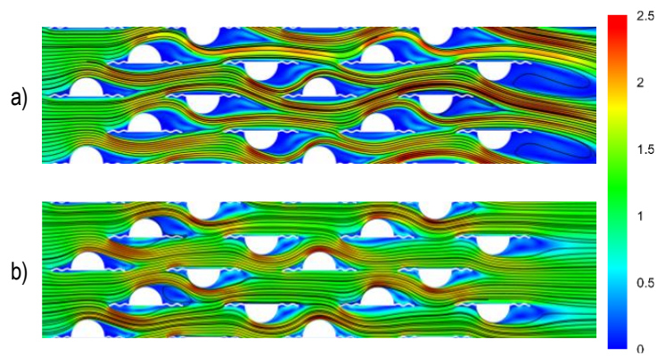
Fig. 6. Streamlines and normalised contours of velocity in finned tube configuration (“2-wave”) for: a) Re = 1,000, b) Re = 10,000
Joining the fins together causes a separation of the flow to the streams that do not mix with each other until leaving the middle section. There are visible slight recirculation regions or even areas where the high-velocity streams omit the long parts of the fins behind the tubes. This layer separation may lead to a deteriorated level of heat exchange between the fins and fluid. On the other hand, the regions of recirculation of the low velocity at the flat part of the tubes are much smaller than in the plain tube case. For the higher Reynolds number, the normalised velocity distribution becomes more uniform.
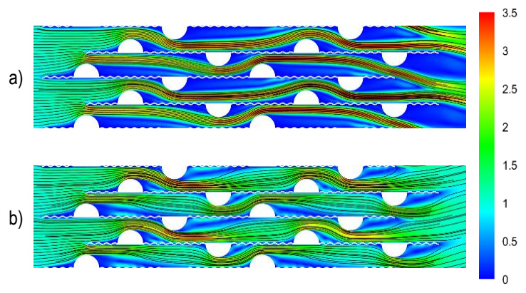
Fig. 7. Streamlines and normalised contours of velocity in finned tube configuration („joined”) for: a) Re = 1,000, b) Re = 10,000
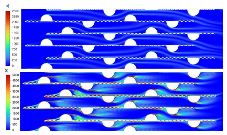
Vorticity contours for the “joined” case are presented in Fig. 8. Values in legends were cropped to present the phenomena more clearly. The maximum reached and visible on contour values were up to around 10,000 s-1 and 30,000 s-1 for Re=1,000 and 10,000, respectively. The recirculation right before and behind the tubes is visible, with the biggest intensification in the first rows. Red long streams are noticed along the peaks of the fins and at the top of the tubes, indicating the boundary layer separation. The recirculation zones are presumably responsible for the increase in pressure losses discussed in the next chapter. At the same time, the side of the fin exposed to intense recirculation between its peaks is simultaneously washed by the high-velocity stream. In these regions, the total surface heat flux is significantly higher compared to the opposite side of the fin, where recirculation is weaker and the high-velocity stream is absent. For example, fins in the third row on the side subjected to both intense recirculation and high-velocity flow reached, on average, a heat flux of 9,700 W/m² at their peaks, and only 4,300 W/m² at the valleys. For fins in a region characterised by overall lower recirculation intensity, the corresponding values were almost halved, reaching 5,600 W/m² and 2,300 W/m², respectively. On the flat portion of the tube, recirculation was relatively weak, and the resulting heat flux was, consistent with the previous comparison, ranging from 2,572 W/m² in the vicinity of the first fin wave to 4,472 W/m² in the middle.
Pressure and friction factor
The static pressure drop versus Reynolds number is shown in Fig. 9a). Each of the curves relates to the various lengths of the wavy fin, which is incremented from 0 waves (plain tube) by one wavelength till the individual fins are long enough to connect (join) to create the continuous plate-fin. The obtained results follow the power function and can be represented as 6·10-07·Re2.034 for the “joined” case, 6·10-07·Re1.964 for the “2-wave” case, and 5·10-07·Re1.946 for the unfinned tubes. Plain tube geometry is characterised by the lowest pressure drop. As more heat transfer surface area is added (increasing fin area), the pressure losses increase. One can see a significant rise in values between when the fin length is increased by more than two wavelengths (“3-wave” and “joined” cases). Pressure drop for the maximum Reynolds number is near 30 Pa for the plain tube case. There is a considerable increase for 1-2 wavelength fins to approximately 40 Pa (a few Pascals of difference between these two geometries). Yet for the increase from two to three fin waves, the maximum Δp increases to approximately 65 Pa. A continuous fin geometry delivers a drop of nearly 85 Pa, increasing the plain semicircular tube result by 188%. The pressure loss may be decreased by changing the distance between the tubes, according to [25]. It may also be mitigated by gradually increasing the first wave’s or fin section’s amplitude until it reaches the desired dimension, to reduce disturbances and limit flow separation at the entrance to the tube bank.
Further reduction of the pressure drop data can be seen in Fig. 8b), where the friction factor is calculated according to:

and is plotted against the Reynolds number. The friction factor for a plain tube bundle is the lowest, with a slightly decreasing trend (from approximately 0.25 to 0.2) within the considered Reynolds number range. For geometries with added fins, one can observe different characteristics, as there is a local minimum visible at a Reynolds number of 2,000. It can lead to the conclusion that for Re = 1,000, the flow is dominantly laminar, as the sharper linear decrease can be seen, and after the transition to turbulent, a milder variation with Reynolds number occurs. Depending on the geometry, a slight decrease or increase is noted, excluding the three-wave-fin, for which, for Re > 3,000, the friction factor stays virtually constant. The considerable rise in the pressure drop in Fig. 9a) from 2 to 3 wavelengths of fin is reaffirmed by the friction factor characteristics. The considerable change in friction factor from 2 to 3 wavelengths of fin geometry indicates a significant change in flow characteristics.
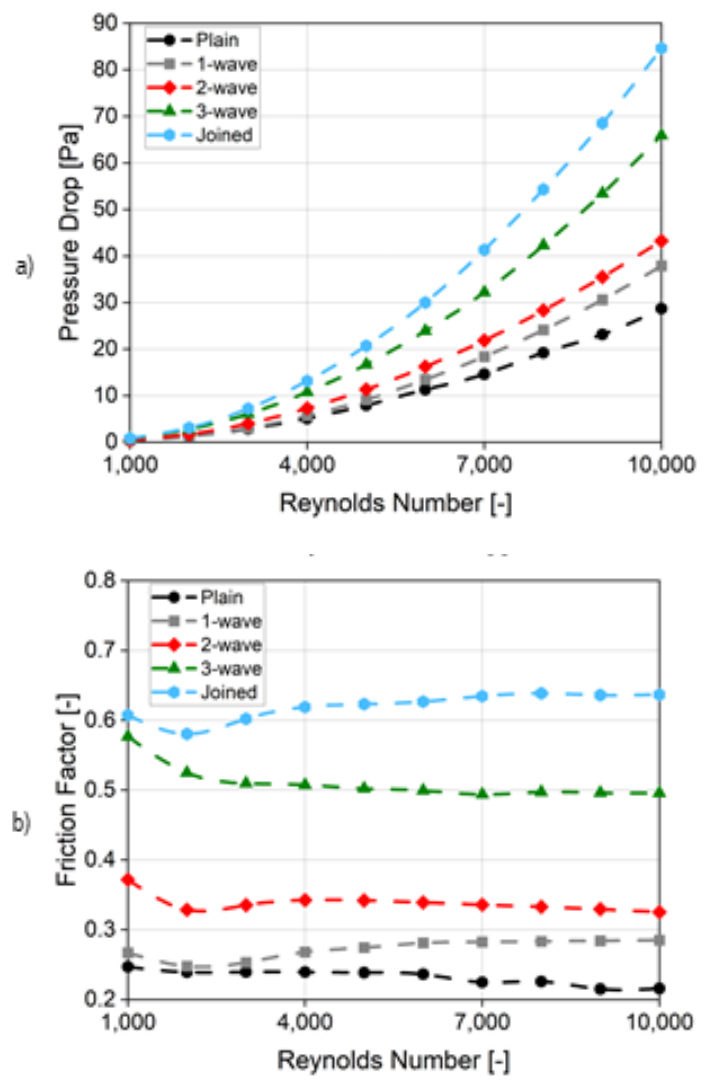
Fig. 9. Results of a) static pressure drop and b) friction factor versus Reynolds number for different fin geometries
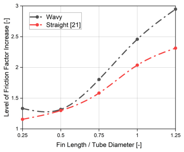
Fig. 10. Level of increase in friction factor between plain and finned tubes at Re = 10,000 for different lengths of fins, wavy and straight fin comparison
In the article by Afifi et al. [21], the level of increase between the finned and plain tubes was compared for different lengths of the fins. They investigated straight rectangular fins connected to the semicircular tubes. Comparing their presented data with the ones obtained, and extrapolated to correlate with the fin lengths, in this study, it was possible to create a graph shown e.g. in Fig. 10. The reached values for Re = 10,000 indicates less favourable results for wavy fins. The trend of difference in friction factor is high at the shortest fin length (15%), decreases at 0.5 fin-to-diameter ratio, to increase again for larger ratios. The maximum losses are larger by even 27% than the straight fins in the case of joined fins. However, for the fin-to-diameter ratio equal to 0.5, the results are comparable (1.5% difference) for straight and wavy fins.
Thermal performance
In Fig. 11, panel (a) shows the heat-transfer rate per unit span of the investigated geometry (per 1 m), while panel (b) presents the non-dimensional heat-transfer rate normalised by that of plain semicircular tubes, plotted versus the Reynolds number. The heat transfer rate correlation for every geometry follows a power-law trend and can be represented as 2.84·Re0.855 for the “joined” case, 5.78·Re0.747 for the “2-wave” case, and 6.28·Re0.687 for the unfinned tubes. The lowest value is obtained for the plain tubes. For every incremental elongation of the wavy fin, thermal performance grows proportionally and is almost constant for the investigated Reynolds number range. The only exception is for the “joined” case. For the tube with a three-wavelength fin, there is a small increase in the heat transfer rate, and only for the conditions of Re > 5,000. There is almost no increase in the exchanged thermal power for the lower values of Reynolds number.
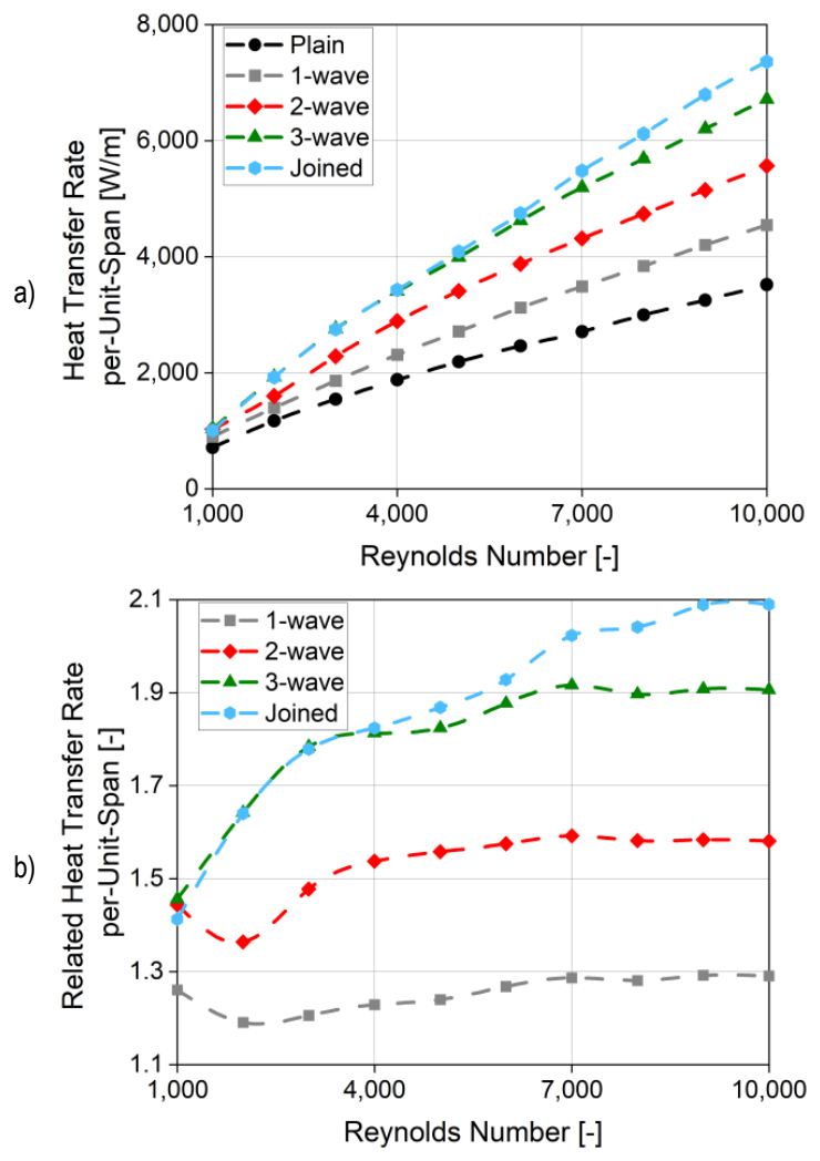
Fig. 11. Heat transfer rate per-unit-span a) and its relation to plain semicircular case b) as a function of Reynolds number for various fin lengths
The joined fin is not a favourable design because an increase in heat transfer is slim with a high rise in the flow resistance. It is additionally visible that the curves for “3-wave” and “joined” overlay each other for Re < 5,000. Regarding the 3 wavelengths fins and shorter, adding a fin of one wavelength causes a rise of 25-30% in heat transfer rate. The curves of cases with fins of one and two wavelengths follow a similar pattern. Below Re = 3,000, the related heat transfer rate decreases linearly, reaches a local minimum and then increases to an approximately constant value from Re = 5,000. For “3-wave” and “joined” cases, the related heat transfer rate grows monotonically: it is steep and almost linear at Re < 3,000, while for higher Reynolds numbers, the slope of the function is smaller. The highest intensification occurs for the largest heat transfer area, and it is equal to 210%.
In the case of the heat transfer rate, the wavy fins are a more favourable option than the straight fins at Re = 10,000 (Fig. 12). The difference between the two geometries increases with the rise in the length of the fins. It reaches its maximum of 22% when the fin is the same length as the tube diameter (fin-to-diameter ratio equal 1). Above this length, the difference decreases to around 20% in the investigated range. The minimum improvement occurs at 0.5 fin-to-diameter ratio, reaching 10%, and it correlates with the lowest value of friction factor difference. The level of increment between the wavy and straight fins connected to the semicircular tubes is shown in Table 2.
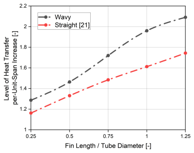
Fig. 12. Level of increase in heat transfer rate per-unit-span between plain and finned tubes at Re = 10,000 for different lengths of fins, wavy and straight fin comparison
Tab. 2. Comparison between wavy (subscript ) and straight (subscript ) fins of reached level of increment in relation to plain semicircular tubes in terms of friction factor and heat transfer
| Fin-to-diameter ratio | Friction factor / | Heat transfer rate / |
|---|---|---|
| 0.25 | 1.15 | 1.11 |
| 0.5 | 1.01 | 1.10 |
| 0.75 | 1.14 | 1.16 |
| 1 | 1.21 | 1.22 |
| 1.25 | 1.27 | 1.20 |
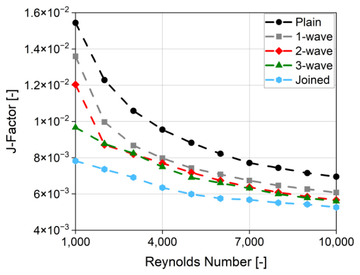
An increase in heat transfer rate appeared in parallel with an increase in pressure drop. To assess the “goodness” of the implemented heat exchanger’s geometry modifications, non-dimensional j- and JF-factors were prepared. Colburn j-factor determines heat transfer in a heat exchanger with respect to Reynolds, Nusselt and Prandtl numbers. The j-factor formula was used as Eq. (8) states:

Differences between the gathered results of heat transfer rate (Fig. 11a) and the ones from Fig. 12 are noticeable. J-factor for all finned cases is shown to have worse characteristics than plain semicircular tubes (Fig. 13). This phenomenon is especially visible at lower investigated Reynolds numbers. Application of the fins increases the heat transfer rate, but they also increase the circumference (surface area) of the investigated object. Following Eq. (3) and (5), the total object’s circumference is one of the components determining the average heat transfer coefficient, then used to calculate the Nusselt number and, ultimately, the j-factor. This and the lower increase of heat transfer rate with the Reynolds number rises were specified as the main reasons for the Nusselt number decrease. A general j-factor decrease along with a larger Reynolds number was also observed in the literature, and it is typical for convective heat transfer. Description of both experiments conducted by Che and Elbel [27] over a staggered finned circular tube heat exchanger and numerical investigation of a microchannel heat exchanger by Kemerli and Kahveci [28] shows a similar trend of the j-factor diminishing exponentially.
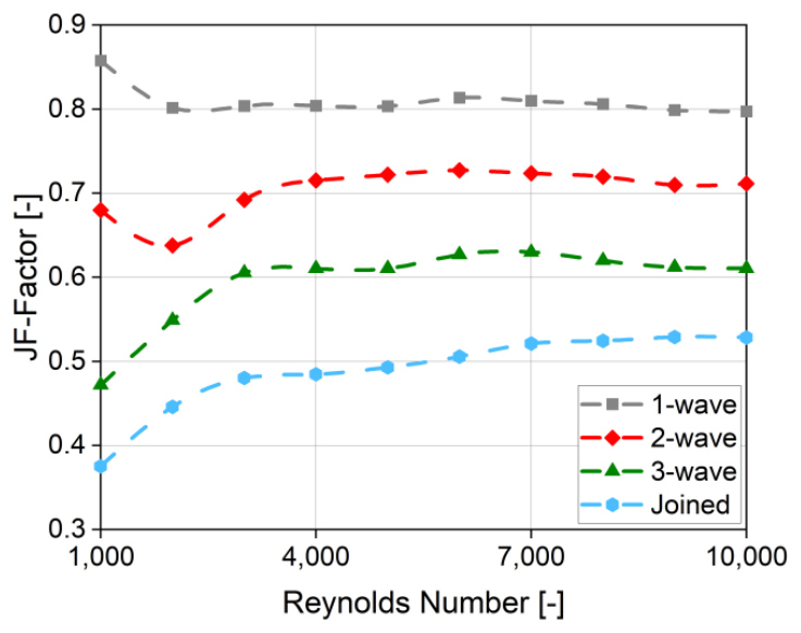
Considering also the friction factor (f-factor), it is possible to compare modifications of the heat exchanger, assessing heat transfer intensification regarding pressure drop penalty. Such a factor is called the JF-factor, and it is a comparative factor to an unmodified case, calculated with Eq. 9. This work considered the plain semicircular case as the benchmark (jref and fref) and the result of the comparison is shown in Fig. 14. The values above 1 would indicate a general thermal performance improvement, and below 1 a general deterioration in characteristics.

It can be noticed that none of the investigated cases reached a value higher than 1. The highest obtained JF-factor was for the case of “1-wave” and was equal to more than 85% of plain semicircular tubes. Having reached its maximum, the value for this case remained stable at around 80% for the next investigated Reynolds number. The lowest factor values, down to less than 40%, were obtained for the joined fins. The final comparison of wavy finned tubes indicates that every elongation of the fin by one wavelength decreases the overall performance by around 10%pt of the “plain” case. The effect of increased friction factor is significantly higher than the potential improvement in heat exchange. This leads to a trade-off, which may not be suitable for applications with limitations of low pumping power. In such a situation, it may be worth considering the case with a single wavelength at low inlet velocity, as it characterises with higher heat transfer rate and almost 0.9 JF-factor.
Local Heat Transfer Coefficient
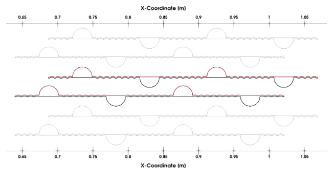
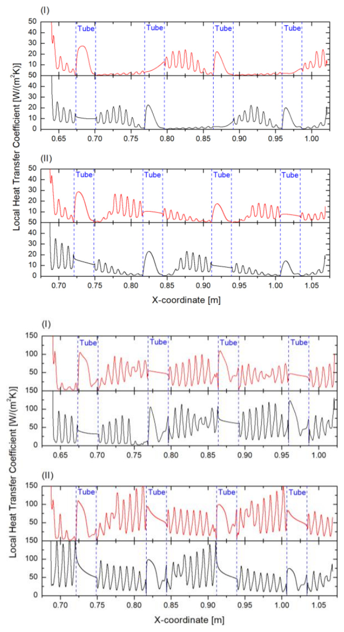
A local Heat Transfer Coefficient (Eq. 10) indicates what is the influence of the region on the overall thermal performance. Three geometries are shown with their description of location on the x-coordinate: plain semicircular tubes (Fig. 15 and Fig. 16), fins of two wavelengths (Fig. 17 and Fig. 18) and the joined fins (Fig. 19 and Fig. 20). Heat Transfer Coefficient (HTC) distributions on these geometries are divided into the upper part marked in red and on the top of the graph, the bottom part of the geometries marked in black and on the bottom of the graph, and calculated HTC values for the lowest a) and highest considered b) Reynolds number. The investigated layout of tubes is a staggered configuration, and thus, the additional division of the graph into the odd (I) and even (II) rows is applied.
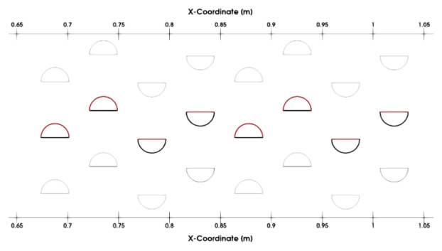
Fig. 15. Modelled geometry with distinguished locations (red – top, black – bottom) at which the local heat transfer coefficient is measured, plain tube case
The heat transfer is the most intense at the stagnation point occurring in the vicinity of the front of the tube (Fig. 5 – Fig. 7). The HTC scale was thus clipped at that point to keep the values within a limited range. This adjustment ensures that the plot resolution is sufficient to examine the data accurately.

where q(x,y) is the local heat flux.
For the plain semicircular tubes, the HTC is at maximum at the leading edge and for the semicircular part of the tube. At Re = 1,000, the highest value of around 90 W/(m2K) is obtained for all the tubes of the odd rows except the first one, at the connection between the flat and curved part of a tube. At Re = 10,000, there is a maximum of around 220 W/(m2K) for the same locations, but at the last one, the value is smaller, equal to 210 W/(m2K). The similar peaks in local HTC have also been noted in the article by Afifi et al. [21], in which the highest value was obtained for the next-to-last row. At Re = 1,000, the tube curvatures exhibit regions of high HTC values at the front, with a steep decrease to a minimum near the trailing edge, followed by a sharp peak at the trailing edge, where the HTC is maximised at approximately 20 W/(m² K). It slightly changes at Re = 10,000. The HTC still decreases downstream of the peak at the front, but it typically recovers to 40% of maximum at 75% of the tube’s diameter. The minimum corresponds to the boundary layer separation point at the middle of the diameter. The HTC values at flat faces at Re = 1,000 stay approximately constant, while at Re = 10,000 grow with further distance for all tubes in the bundle. This phenomenon can be explained by the smaller and flatter separation bubble for the higher Reynolds number, as visible in Fig. 5 – Fig. 7. For certain tubes, the re-attachment of the boundary layer can be clearly observed at approximately ¾ of the diameter.
As can be seen from the geometry given in Fig. 17, as the tube is no longer the leading element in contact with the flow, the local HTC distributions differ (Fig. 18). There are visible fluctuations that correspond to the wave-fin curvature. The peaks are displaced to the leading edges of the fins. The highest reached HTC is approximately. 180 W/(m2·K) for the upstream of the second tube’s fin in both odd- and even-tube rows at Re = 1,000, and around 500 W/(m2·K) at Re = 10,000. It can be explained by the presence of higher velocity streams that are created downstream of the first rows as a result of the flow area contraction (Fig. 6). At the bottom part (especially fins) of every geometry at Re = 10,000, heat transfer is intensified with respect to the plain tube case. It can be associated with the fact that the highest Reynolds number low velocity regions are flatter and smaller at the flat half of the finned tube than for the plain tube. Whereas the HTC values at the round and flat parts of tubes at Re = 1,000 are virtually unchanged. However, at Re = 10,000, the flat parts are also characterised by a flat distribution of local HTC, except for the first tubes in both odd- and even-tube rows, where an increase can be observed.
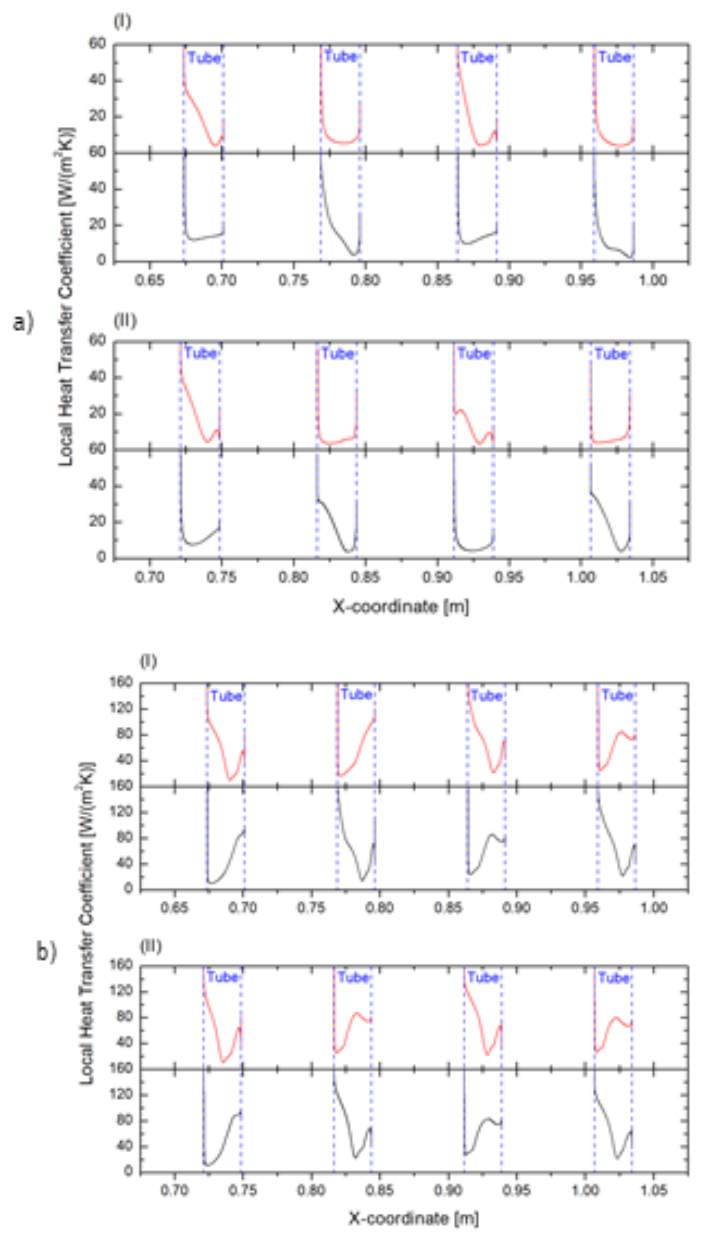
Fig. 16. Local heat transfer coefficient results with respect to x-coordinate at Reynolds number equal to a) 1,000 and b) 10,000 for (I) odd tube rows, (II) even tube rows; plain tube case
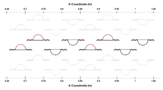
Fig. 17. Modelled geometry with distinguished locations (red – top, black – bottom) at which the local heat transfer coefficient is measured; “2-wave” case
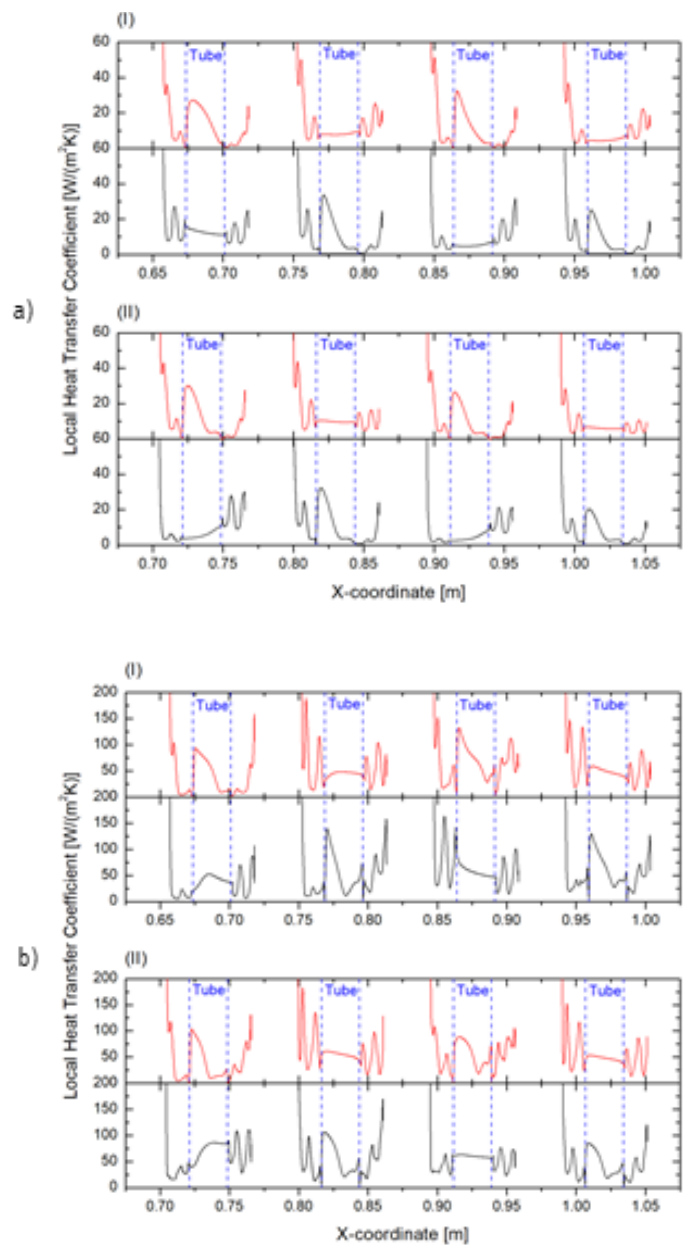
Fig. 18. Local heat transfer coefficient results with respect to x-coordinate at Reynolds number equal to a) 1,000 and b) 10,000 for (I) odd tube rows, (II) even tube rows; “2-wave” case
The joined fin causes the flow to be separated into a few high velocity streams, as it was shown in Fig. 7. The effect of those streams is visible in the HTC graphs (Fig. 20). At Re = 1,000, the fins at which the flow stagnates or even omits them, it is clearly seen that a very low value of the local HTC. As it is shown, the fins of the odd-row tubes in the middle have a very low thermal efficiency. The maximum values of HTC are not obtained only at the leading edge of the fins, but also in the middle. The highest values of HTC are reached at the tip of the fin in the even-tube-row and are equal to around 11,700 W/(m2·K) at Re=10,000, and at Re = 1,000 to around 31,000 W/(m2·K). They occur only on very few elements at the tip of the fin and were considered as the numerical artefact. These also significantly differ from the obtained values further downstream. Thus, the graphs have been cropped to values that ensure the clarity of the readings. At Re = 1,000 HTC is up to around 30 W/(m2·K), while at Re = 10,000 up to 150 W/(m2·K).
Temperature
Contours of the normalised temperature distribution (Eq. 11) are presented in Fig. 21 – Fig. 23. They clearly visualise what the effect of the applied modifications is on the crucial function of the heat exchanger, which is changing the fluid stream temperature. Following the equation, the value of one is obtained at the tubes’ surface, where Ts = 400 K – constant temperature boundary condition is specified. Zero indicates regions of minimal temperatures from the inlet (Tin) – 300 K.

Comparing all the figures, the application of fins causes an improved heating of the fluid. The highest temperature areas are especially present in the vicinity of the tubes and areas where the stagnation of the flow happens. On the other hand, the inlet temperature pertains in the jets until the mixing at the outlet of the middle section. There, they get in contact with the hotter streams, and the temperature is distributed in the outlet section until it is evenly distributed at the outlet. An increase in the inlet velocity causes a decrease in the bulk outlet temperature. It is a phenomenon clearly caused by the shorter time of contact between the heat source and fluid.
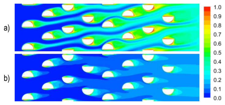
Fig. 21. Normalised contours of temperature in plain tube configuration for: a) Re = 1,000, b) Re = 10,000
Fins visibly enlarge the regions of maximal temperature in the contour maps. This is caused by increased area of contact between the fluid and the hot elements, which is supported in heat transfer rate graphs (Fig. 11), by generally higher heat transfer rates. At Re = 1,000, clearly visible high-velocity, cold streams from plain tubes case (Fig. 21a) reaching the end of the bundle, are in the “2-wave” case at the Tnorm≈ 0.3 (Fig. 22a).
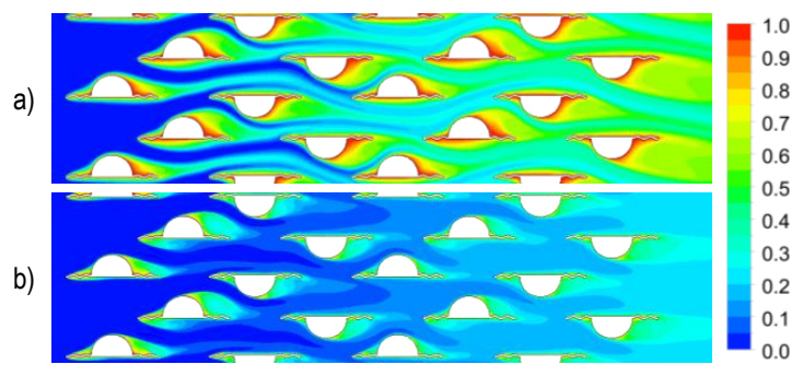
Fig. 22. Normalised contours of temperature in tube with two-wave-fin configuration for: a) Re = 1,000, b) Re = 10,000
The “joined” case is characterised by a clear separation of the streams. Even though the fins are used, the cold stream reaches the next-to-last tube for Re = 1,000 (Fig. 23a), which is caused by the mentioned separation of flow. Additionally, there appear to be many hot regions in the middle section, but they are the stagnated regions, which are characterised by poor heat transfer.
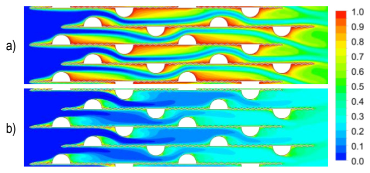
Fig. 23. Normalised contours of temperature in tube with joined fin configuration for: a) Re = 1,000, b) Re = 10,000
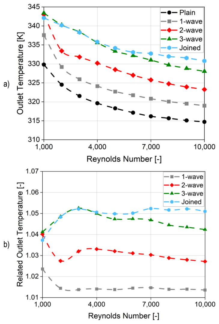
Fig. 24. Outlet temperature a) and its relation to plain semicircular case b) as a function of Reynolds number for various fin lengths
The reached outlet temperature and the relationship between the values for finned and plain cases are shown in Fig. 24. A notable observation is that at a Reynolds number (Re) of 1,000, the outlet temperature is reduced for the joined fin configuration relative to the two-wavelength fin. A further increase in the Reynolds number results in a decline in the outlet temperature across all tested configurations. The “3-wave” and “joined” cases deliver very similar results until Re = 4,000. At higher Reynolds numbers, the temperature becomes greater for the “joined” case. This behaviour is like that exhibited by the heat transfer rate seen in Fig. 11. The highest temperature reached is for the “3-wave” case at Re = 1,000, at around 343 K. The lowest was for plain tubes at Re = 10,000, at approximately 315 K. Application of the fins consistently resulted in higher outlet temperatures than for the plain tube bundle. The most significant improvement was at Re = 3,000 and 7,000, where the “joined” case increased the temperature by 5.2% compared to the plain tube bundle. The smallest improvement was 1.4%, observed with the shortest “1-wave” fin geometry.
CONCLUSIONS
The article presents the results of conducted simulations for a geometry of a semicircular tube bundle with longitudinal wavy fins. The changed parameters were the length of the fins (from plain tubes to the joined fins) and the inlet velocity (in the Reynolds number range of 1,000-10,000). The main conclusions from the research performed are:
Similar to the experiments over straight fins [21], the elongation of wavy fins leads to a rise in all considered output parameters. The highest reached values of local velocity, pressure drop, and heat transfer rate were for the case of joined fins. The tubes with fins of three wavelengths delivered similar results, especially at lower Reynolds numbers.
Applying fins causes the appearance of regions with elevated normalised velocity, to 3.5 against 2.5 for plain tubes.
The lowest friction factor (0.2-0.3) was reached for a bundle of plain tubes and with a fin of one wavelength. The joint fin case was characterised by a twofold increase.
The most favourable geometry regarding heat transfer rate is the joined fin, especially for Reynolds numbers between 9,000 and 10,000. Applying such fins doubles the heat transfer rate with respect to the plain tubes. For Re < 5,000 tubes with fins of three wavelengths yielded similar results.
The wavy fins improve the heat transfer rate by a maximum of 22% in comparison to the straight fins. However, this improvement relates to the friction factor rise by up to 27%.
The highest Colburn j-factor (1.6·10-2) was reached for a bundle of plain tubes at the lowest inlet velocity. The joined fin case was characterised by its twofold decrease.
The JF-factor, combining thermal performance and the flow resistance, shows a 10%pt decrease for every wavelength elongation in comparison to the plain semicircular tubes. The best modified case was with one wavelength of fin, which delivered around 80% of the plain tubes throughout the whole studied Reynolds number range.
The significant difference between HTC values at the concave and convex parts of the fins suggests that the fin area could perform with a higher thermal effectiveness after further fin geometry modification.
Applying wavy fins can increase the outlet temperature by up to approximately 5%. The “joined” case suffers from flow separation and many stagnation zones that do not allow the system to work on its “full capability”. The “joined” and the “3-wave” cases deliver similar temperatures at the outlet for the whole investigated Reynolds number range.
The semicircular tubes in connection with the longitudinal wavy fins can be a useful solution in heat exchangers requiring maximisation of the heat transfer rate. The authors believe that further research on such fin modification can point out an even more effective geometry in thermal-flow characteristics. The other geometries may employ fins with various wave amplitudes or with a different profile, similar to the article of J. Dong et al. [26]. The current work may play role as a benchmark for a parametric study concerning the number of waves or their amplitude. It could be worth finding the effect of the fins’ angle of attack on the measured parameters, applying different materials and assessing the economic factors of production of such heat exchangers. Having investigated these elements, it is suggested to perform experimental studies of the novel geometries.