1. INTRODUCTION

Nanocomposite materials reinforced with carbon nanotubes are now widely used in engineering due to their exceptional physical properties [1–4]. Carbon nanotubes can be divided into single-walled nanotubes (SWNT), which typically have a diameter of 0.8 to 2 nm, and multi-walled nanotubes (MWNT), which have a diameter of 5 to 20 nm. Carbon nanotubes can vary in length from less than 100 nm to several centimeters, and their ends can be open or closed. CNTs are characterized by a high stiffness modulus of approximately 1000 GPa, tensile strength of 100 GPa, and low density [5]. They are highly resistant to large bending deformations and return to their original shape without damage. The high aspect ratio of CNTs and the large interfacial area result in effective load transfer from the matrix to the nanotubes. The use of fibers in a composite with a stiffness greater than that of the matrix increases the stiffness and strength of the material [6–8]. The interaction between the matrix and the nanotubes increases the damping of the material. Nanocomposites can absorb mechanical energy. Inclusion of nanotubes increases fatigue strength and fracture resistance. In addition to their excellent mechanical properties, nanocomposites are characterized by good thermal conductivity, stability, and resistance to heat and environmental factors. They also have the property of shielding and absorbing electromagnetic waves.

The exceptional mechanical, thermal, and electrical properties mentioned above have led to the use of nanotube-reinforced polymers in the automotive industry for the production of exhaust system components, catalytic converters, suspension and braking systems, engines, and body parts. Another area of application is aviation. Nanocomposites are used as components of wings and fuselages. A new area of application is sports equipment, e.g., badminton and tennis rackets, baseball bats, bicycle frames, etc. Carbon nanotubes are used to reinforce composites used in wind turbine blades and hulls of maritime boats [5][9–11]. In many of the applications mentioned, nanocomposites are dynamically loaded.

Efficient analysis of displacement, strain, and stress fields in dynamically loaded composites containing a large number of fibers requires the use of experimental or computer methods. Richardson and Wisheart [12] showed a review of the definitions of low-velocity impact and modes of failure of composites (matrix and fiber failures, delamination, and penetration). The influence of the composites constituents on impact response and post-impact residual strength was analyzed. Liu et al. [13] analyzed orthotropic birefringent composites subjected to impact loading using photoelasticity, strain measurement, and the time-domain boundary element method to calculate dynamic material constants, stress-fringe values, and to verify the stress-optic law. Different directions of the material axes with respect to the applied uniaxial and biaxial loading were considered. Residual stresses were taken into account. Malekzadeh and Zarei [14] analyzed the natural frequencies of quadrilateral laminated plates reinforced with carbon nanotubes. The composite material was homogenized using the extended rule of mixture. The governing equations based on the first-order shear deformation theory of plates were transformed from an arbitrary physical quadrilateral domain to a computational square domain. The spatial derivatives in the equations were discretized using the differential quadrature method (DQM). They studied the convergence of the DQM method, the influence of the geometry of the plate, the orientation of layers, the distribution of nanotubes, and the support conditions on natural frequencies. Phung-Van et al. [15] applied isogeometric analysis (IGA) based on non-uniform b-splines (NURBS) and higher-order shear deformation theory to analyze static and transient deflections, natural frequencies and mode shapes of rectangular and circular functionally graded carbon nanotube-reinforced plates. The plate material was homogenized using the rule of mixtures. They analyzed the influence of the parameters of the IGA method, the geometry of the plates, the distribution of the nanotubes, the support conditions, and the time variation of the loads on the response of plates. Rasoolpoor et al. [16] presented the analysis using the finite element method of a hybrid polymer composite reinforced by carbon fibers and carbon nanotubes subjected to low velocity impact. The influence of microstructure and dimension of composite, support and impact conditions, number of finite elements, on time variations of dynamic contact forces and deflections of the plates was studied. Tarkashvand et al. [17] presented an analytical method to analyze a complex problem of the vibroacoustic response of the CNT-reinforced composite shell. The structure was resting on an elastic foundation and was submerged in a moving fluid, thermally loaded, and excited by an acoustic plane wave. They studied the influence of parameters such as elastic foundation, temperature gradient, CNT distribution, and Mach number.

An important issue is the accurate modeling and analysis of single carbon nanotubes. Tserpes and Papanikos [18] presented a three-dimensional finite element model for single-walled carbon nanotubes. The parameters of the beams were determined by comparing the energies calculated using molecular mechanics and continuum mechanics. The influence of wall thickness, diameter, and chirality of nanotubes on elastic moduli was investigated. Li and Chou [19] presented single-walled carbon nanotubes subjected to harmonic waves. The velocities of the longitudinal, transverse, and torsional waves were calculated using the molecular mechanics and mode superposition method. They analyzed the influence of nanotube diameter, chirality, and wave frequency on wave propagation. Sakhaee-Pour et al. [20] modeled single-walled carbon nanotubes using three-dimensional elastic frames and concentrated masses. The atomistic finite element method was used to calculate natural frequencies and mode shapes for zigzag and armchair configurations, different diameters, lengths of nanotubes, and boundary conditions. The results were approximated using a predictive equation. Khalili and Haghbin [21] modeled single-walled carbon nanotubes embedded in a polymeric matrix as space frames using FEM. The geometrical and elastic properties of the beam elements were obtained by comparing the potential energy in molecular mechanics with the strain energy in structural mechanics. The influence of the volume fraction, diameter, and chirality of the nanotubes on axial strains and the strain energy density of nanocomposites subjected to impact tensile loads was studied.

Usually, nanocomposites are modeled using computer methods to calculate the effective mechanical properties by considering a representative volume element (RVE). Thostenson and Chou [22] derived the equation for the effective elastic properties of polystyrene composites reinforced with multi-walled aligned carbon nanotubes. They experimentally measured geometric parameters of nanotubes: diameter, length, orientation, and mechanical properties to calculate effective properties of nanocomposites. Tsai et al. [23] modeled CNT/polyimide nanocomposites as cylindrical solids. The elastic properties were calculated using molecular dynamics in conjunction with the energy equivalence concept. The atomistic interaction between the CNTs and the polyimide polymer matrix was modeled as an effective interphase. The micromechanical properties in the longitudinal and transverse directions of the nanocomposites were compared with the results obtained by the Mori-Tanaka model and by the molecular dynamics. Tserpes and Chanteli [24] evaluated the effective properties of multi-walled carbon nanotube reinforced polymer composites using a three-dimensional FEM model of RVE. The influence of the properties of the nanotube material, the aspect ratio, volume fractions, interface thickness, and stiffness was analyzed. The results on the microscale were used to predict the tensile modulus of the composite with randomly aligned nanotubes. The numerical results were compared with the experimental data presented in the literature. Chwał and Muc [25] used FEM and an RVE to investigate the effect of the distribution of parallel single-walled carbon nanotubes on the equivalent elastic properties of a polymer matrix composite with nanotubes. The results obtained for the transversely isotropic model of the composite were compared with those obtained by micromechanical analytical methods.

If the stiffness of the fibers is much higher than that of the matrix, then the modeling of the composite can be simplified by assuming that the fibers are perfectly stiff. Pingle et al. [26] used the duality principle to analyze stresses in the vicinity of rigid line inclusions and the compliance of the composite. Pike and Oskay [27] presented the application of the extended finite element method (XFEM) with a new enrichment function for two-dimensional models of composites with random short and rigid fibers. The motion of the rigid fiber was modeled by constraining the displacement field along the fibers. The method was used to study the influence of the weight fraction of fibers on the effective Young modulus.

The boundary element method is a general computer method that has also found application in nanocomposite mechanics. Liu et al. [28] used the fast multipole boundary element method (FMBEM) to analyze the effective elastic properties of carbon nanotube reinforced composites. The composites were modeled as three-dimensional structures containing a very large number of rigid fibers. The perfect connection between the rigid fibers and the elastic matrix was assumed. The stress distributions at the fiber-matrix interfaces and the influence of the volume fraction of fibers on effective Young’s modulus were studied and compared with the available results reported in the literature. Wang and Yao [29] used rigid-fiber-based FMBEM to analyze the interfacial debonding process and the strength of nanotube-reinforced composites. It was assumed to fail when the shear stress reached a limiting value. The solution was obtained using an incremental procedure. The effects of aspect ratio, volume fraction, and number of nanotubes in the RVE on the detachment areas, nonlinear stress-strain curve, and effective Young's modulus were investigated. Yao et al. [30] used the FMBEM to analyze carbon nanotube composites. They assumed that fibers are subdomains having identical geometrical and physical properties. The effects of the aspect ratio of the fibers, the number of fibers, the volume fraction, and also the elastic interfacial conditions or the additional interfacial layer between the deformable fibers and the matrix on the effective Young modulus were investigated.

Fedeliński and Górski [31] applied the coupled finite element and boundary element method to analyze and optimize statically and dynamically loaded plates reinforced by deformable stiffeners. The plates were modeled using the dual reciprocity BEM and the reinforcement by the FEM. The aim of optimization was to maximize the stiffness and strength of the composites by changing the lengths and locations of the stiffeners. The optimal design problem was solved using the evolutionary algorithm. The same approach was used by Fedeliński and Górski [32] to maximize the stiffness of statically loaded nanocomposites with single and two-layer platelet-like particles by changing the distribution of inclusions. Fedeliński [33] used the BEM to analyze plates containing cracks and reinforced with thin, straight, and rigid fibers. The influence of the position of the rigid fibers on the effective properties of the composites and on the crack stress intensity factors was investigated. The same approach was used by Fedeliński [34] to analyze the effective elastic properties of composites with randomly distributed thin, parallel, and inclined rigid fibers.

The aim of this work is to present the formulation and applications of the BEM in the analysis of carbon nanotube-reinforced composites modeled as linear-elastic plates with rigid, thin, and straight nanotubes under impact loads. The perfect connection between the nanotubes and a deformable matrix is assumed. This work is an extension of the previous research by the author on statically loaded composites [33–34]. The boundary integral equations formulated in the domain of Laplace transforms are used to determine the relationship between the time-dependent tractions acting on the matrix and nanotubes and their displacements. In order to analyze the problem using the BEM, the boundaries of the plate and nanotubes are divided into boundary elements. Boundary integral equations are used for the nodes on the boundaries of the plate and nanotubes. The standard system of boundary integral equations is extended by equations of motion of nanotubes. The solution in the time domain is obtained using the numerical inversion Durbin method [35], which has recently been used in several works. Zhang et al. [36] analyzed a beam loaded with a moving load. The effect of load velocity and beam damping on its displacement was investigated. Bakhtiari et al. [37] analyzed wave propagation caused by an impulsive load in two coaxial cylinders made of different materials filled with fluid between them. They studied the influence of material properties and inner cylinder dimensions on stresses in the outer cylinder.

The literature review shows that carbon nanotube-reinforced composites have been analyzed using various computational methods, including the finite element method [16], extended finite element method [27], differential quadrature method [14], isogeometric analysis [15], and others. These methods require discretization and interpolation of mechanical quantities over the whole composite domain. The boundary element method allows for the analysis of carbon nanotube-reinforced composites by dividing only the external surfaces and nanotubes into boundary elements and interpolating mechanical quantities only along these surfaces. This makes it very easy to change the position, dimensions, and discretization of nanotubes and external surfaces. Since mechanical quantities are interpolated only along the boundaries, BEM can give accurate results, especially in the case of large stress variations that occur in composites. In the DQM [14] and IGA [15] methods, the composite material is replaced by an equivalent homogeneous material. In the presented formulation of BEM, each nanotube is modeled, which allows for a detailed analysis of the displacements of the nanocomposite. To the author's knowledge, BEM has only been used to model nanocomposites with rigid fibers that were statically loaded. The overview of modern applications of nanocomposites at the beginning of the chapter shows that many of these materials are dynamically loaded. The original achievement of this work is the presentation of the BEM formulation for dynamically loaded nanocomposites and the investigation of the accuracy of the method. Computer software has been developed by the author that uses the method formulated for dynamically loaded nanocomposites.

The present work shows boundary integral equations in the Laplace domain for a composite with nanotubes, equations of motion of a nanotube, and numerical implementation of the method. The displacements computed by the BEM are compared with the FEM solutions, showing very good agreement. The influence of the number of carbon nanotubes, their configuration, and length on displacements is studied.

2. BOUNDARY INTEGRAL FORMULATION FOR CARBON NANOTUBE-REINFORCED COMPOSITES SUBJECTED TO DYNAMIC LOADS

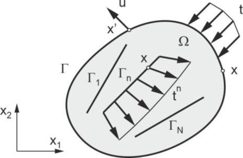
In the present chapter, boundary integral equations for dynamically loaded carbon nanotube-reinforced composites are presented. Initially, only a matrix without nanotubes is considered. The matrix is assumed to be homogeneous, isotropic, and linear elastic. The external boundary Γ of the matrix is loaded by time-dependent tractions t_j, and the domain Ω by body forces f_j. The initial conditions at time t=0 are: the initial displacements u_j = 0 and the initial velocities u˙j=0 The dot over the variable denotes the derivative with respect to time. The relationship between displacements u_j, boundary tractions t_j, and body forces f_j can be expressed by the boundary integral equation formulated in the time-domain [38]:

Eq. (1) can be solved using the time-stepping technique or the integral transform method. In the present work Eq. (1) is transformed using the Laplace integral transform, defined as:

After the transformation, Eq. (1) has the form [39]:

Let us now consider the matrix reinforced by carbon nanotubes, shown in Fig. 1. The mechanical properties of nanocomposite components have been presented in many papers. For example, Thostenson and Chou [22] reported that the most commonly recorded diameter of carbon nanotubes is 18 and 30 nm, their length ranges from 500 to 2000 nm, their average density is 1900 kg/m³, and their Young's modulus is 1000 GPa. In contrast, polystyrene, which is the matrix, has a Young modulus of 2.4 GPa and a density of 1000 kg/m³. In the work of Rasoolpoor et al. [16], it is stated that Young's modulus of carbon nanotubes is 1382.5 GPa, their density is 1300 kg/m³, and the length-to-diameter ratio is 100. In contrast, polyamide, which is the matrix, has a Young's modulus of 4.2 GPa and a density of 1310 kg/m³. Because the stiffness of the carbon nanotubes is much greater than that of the matrix, it is assumed that they are perfectly stiff. The aspect ratio of the nanotube dimensions is usually high. In the present approach, they are treated as thin, straight, and perfectly connected to the matrix. The interaction forces occur between the matrix and the nanotubes because the matrix deforms and the nanotubes are subjected to inertial forces. The interaction forces can be regarded as internal forces fj, shown in Eq. (1), acting on the matrix and distributed only along the nanotubes. Eq. (3) for the matrix loaded by external boundary tractions and the interaction forces have the following form:

Fig. 1.

Matrix reinforced by thin, straight, and rigid nanotubes

The proposed method will be applied to simple cases of external load variability over time, e.g. impact load, rectangular impulse, ramp load, triangular impulse, etc. For this type of load, Laplace transforms can be calculated analytically.

3. DISPLACEMENTS AND EQUATIONS OF MOTION FOR THIN, STRAIGHT, AND RIGID NANOTUBES

The nanotubes change their position and direction in a dynamically loaded nanocomposite, as shown in Fig. 2. It is assumed that the nanotube is thin, straight, and rigid, and the angle of rotation is small. In this case, the components of displacements u_i of the an arbitrary point x of the nanotube are:

Fig. 2.

Displacements of the nanotube (dashed line – initial orientation of the nanotube)

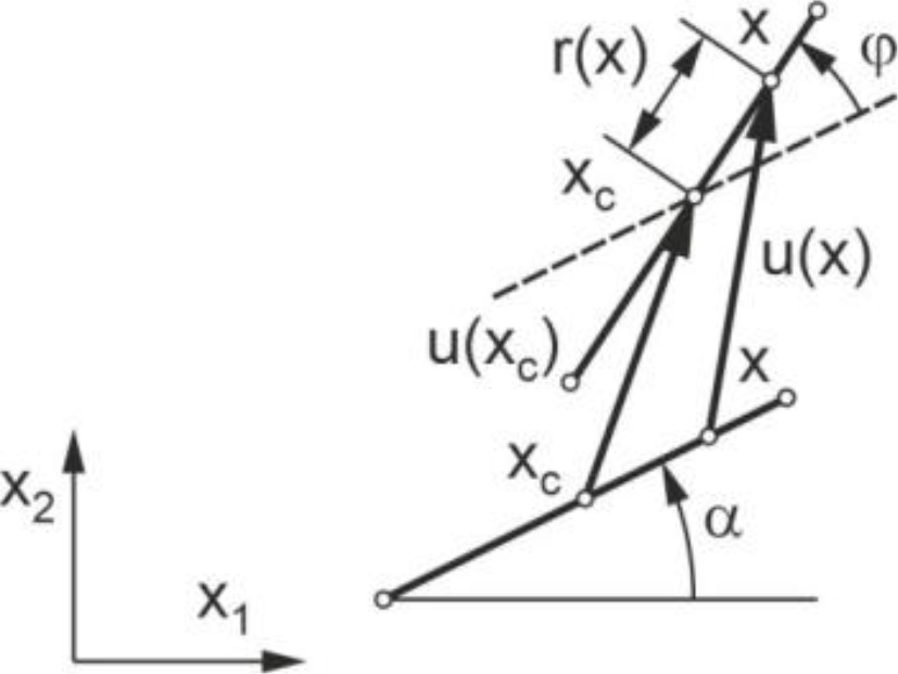
The equations of the motion of the center of the nanotube n have the following forms:

Fig. 3.

Distribution of tractions along the nanotube

The Laplace transforms of Eqs. (7), (8) and (9) are:

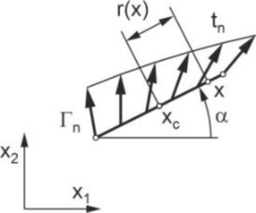
4. BOUNDARY ELEMENT FORMULATION FOR A COMPOSITE REINFORCED BY CARBON NANOTUBES

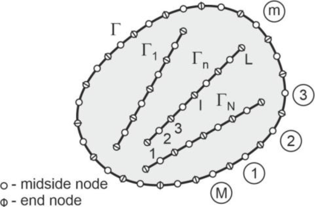
In the present boundary element formulation, only external boundaries and each nanotube are divided into boundary elements, as shown in Fig. 4. As in the standard BEM formulation, the coordinates of points, displacements, and tractions along the external boundaries are interpolated using nodal values and shape functions. The same interpolation is used for interaction tractions along the nanotubes. Because the nanotubes are thin, straight, and rigid, the coordinates of their points can be calculated exactly, and the displacements can be calculated using Eq. (5) and (6). The boundary elements have three nodes, and quadratic shape functions are applied for interpolation.

Fig. 4.

Division of the external boundary and nanotubes into boundary elements

The interpolated quantities are substituted into the boundary integral Eq. (4). The collocation points x’ are all nodes. After the discretization, Eq. (4) expresses the relationship between nodal tractions and displacements. The boundary elements are transformed from the global coordinate system to the local coordinate system, and the integrals are calculated numerically using the Gaussian quadrature. The system of equations for all nodes can be written in matrix form as in the standard BEM formulation:

The dimensions of the submatrices are as follows:

The displacements of the internal nodes, which belong to nanotubes, are expressed by the displacements of their centers using Eqs. (5) and (6). The equations for transformed displacements of all nanotube nodes can be written in matrix form:

The equations of motions (Eqs. (10), (11) and (12)) for nanotube centers can be expressed in the matrix form:

The dimensions of the matrices are as follows:

The displacements of the internal nodes in Eq. (13) are expressed by Eq. (14). The matrix Eq. (13) is additionally extended by the equation of motion of nanotubes (15) giving:

To solve the equation, the submatrices are rearranged. After the modification, the unknown variables are on the left-hand side and the known boundary conditions on the right-hand side of the equation. The unknown transformed internal tractions t_i and the corresponding column are rearranged as follows:

The matrix equation can be solved if the tractions on the external boundary are known. Usually on one part of the external boundary the tractions are known, and on the remaining part, the displacements are given. In this case, the matrices u_e, t_e and the corresponding columns of the matrices H and G are rearranged, as in the standard BEM [38]. The direct solutions of the matrix equation are unknown Laplace transforms of external and internal nodal displacements and tractions. The solution in the time-domain is obtained using the Durbin method [35] of the inverse Laplace transform. For a complete description of the method, Appendix A provides basic information on the Durbin method and the parameters recommended for the method.

In summary, the BEM analysis can be presented in the form of the following flowchart:

5. NUMERICAL EXAMPLES

In this chapter, three numerical examples are considered. The first example, a single nanotube in a rectangular plate, is used to verify the convergence of the method and to investigate the influence of the time variability of loading. The second example, a rectangular plate containing 15 parallel nanotubes, shows the influence of the distance between the nanotubes on the displacements. The third example, a rectangular plate containing 13 parallel nanotubes, demonstrates the influence of nanotube length on displacements. The chapter is completed by an analysis of the influence of reinforcement on displacements and a physical interpretation of the behaviour of nanocomposites.

The matrix is epoxy resin, which is treated as a linear elastic, homogeneous, and isotropic material. The Young modulus of epoxy resin is E=3 GPa, the Poisson ratio is v=0.3, the density ρ=1200 kg/m³ and the plates are under plane stress conditions. Because the nanotubes are very thin and the density of carbon nanotubes is similar to that of the matrix, the inertia of nanotubes is neglected in the present examples.

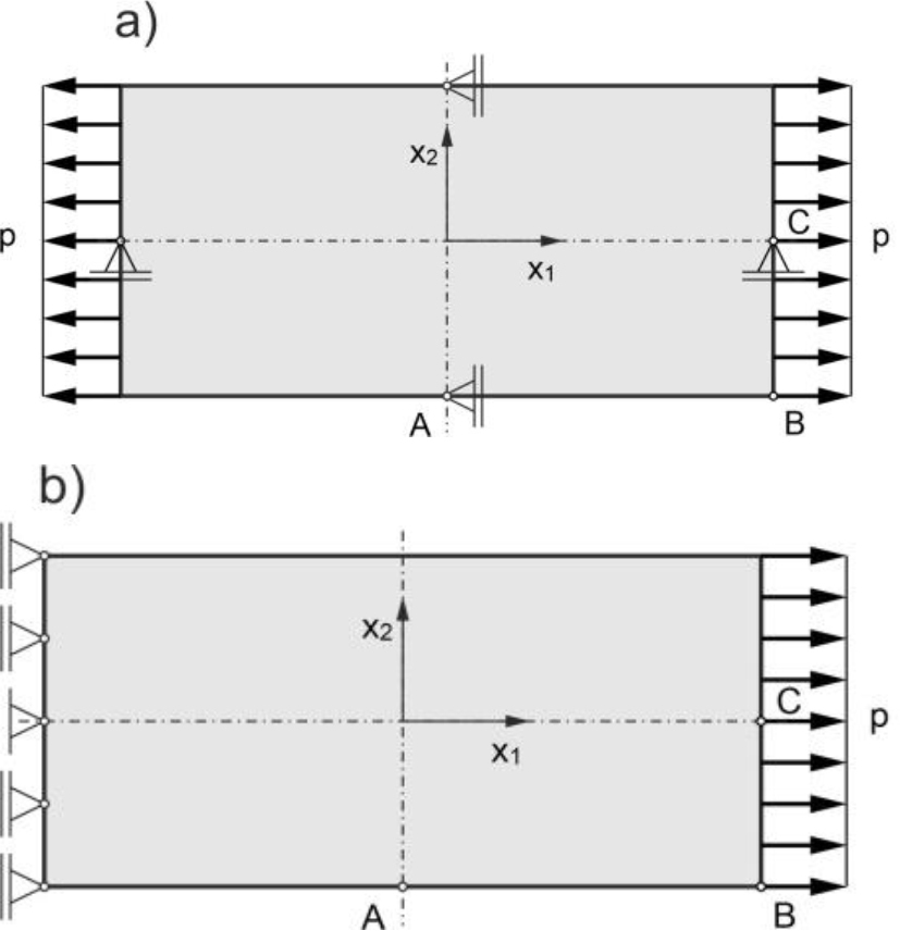
The plates are subjected to two types of boundary conditions, which are shown in Fig. 5. In the first case, the plate is supported on the roller supports along the lines of symmetry and two edges are loaded by the uniformly distributed tractions p in opposite directions. In the second case, the left edge of the plate is constrained using roller supports, and the right edge of the plate is loaded. The load is an impact load with Heaviside time dependence (it is suddenly applied at time t=0 and sustained). The displacements of three selected points A, B, and C shown in Fig. 5 are analyzed. The displacements are normalized with respect to u_o, which is the displacement of point C of the statically loaded matrix without nanotubes. The number of Laplace parameters used in the Durbin method for the numerical inverse Laplace transform is 50. The displacements computed by the BEM are compared with the FEM solutions [40]. In the FEM analyses, the nanotubes were modeled as straight, thin and rigid. This modeling method was implemented by imposing appropriate constraints on the relative displacements of the nodes, resulting in a rigid connection between the nodes lying along the nanotube.

Fig. 5.

Boundary conditions for the plates: a) two-edge loading, b) one-edge loading

Rectangular plate with a single nanotube – influence of time variability of loading

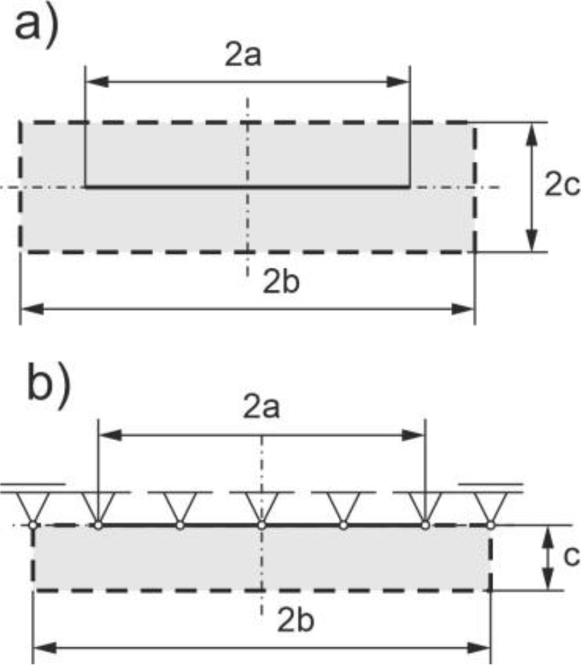
A rectangular plate of length 2b=1.4 μm and height of 2c=0.4 μm contains a nanotube of length 2a=1.0 μm, as shown in Fig. 6a. To verify the accuracy, the displacements of the whole plate and the half of the plate are compared. The half of the plate is supported on roller supports along the horizontal line of symmetry and is additionally fixed along the nanotube, as shown in Fig. 6b. The half of the plate is analyzed using the standard BEM code. The whole plate is divided into 46 boundary elements, and half of the plate into 32 boundary elements, including 10 elements for the nanotube. In the FEM, the whole plate is divided into 224 four-node quadrilateral elements.

Fig. 6.

Rectangular plate with a single nanotube – dimensions of the plate: a) whole plate, b) half of the plate

The components of normalized displacements of selected points for two-edge loading are shown in Fig. 7. The solutions are compared with the displacement of half of the plate and FEM displacements. Very good agreement of the results can be seen in Fig. 7.

Fig. 7.

Rectangular plate with a single nanotube – normalized displacements of selected points for two-edge loading

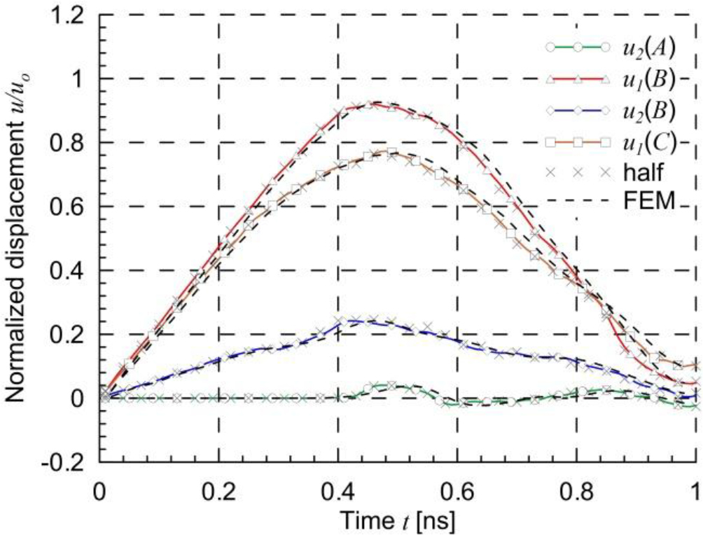
The components of normalized displacements of selected points for one-edge loading are shown in Fig. 8. In this case, the half plate cannot be used for the comparison because the nanotube moves in the horizontal direction. Very good agreement of the BEM and FEM results can be seen in Fig. 8.

Fig. 8.

Rectangular plate with a single nanotube – normalized displacements of selected points for one-edge loading

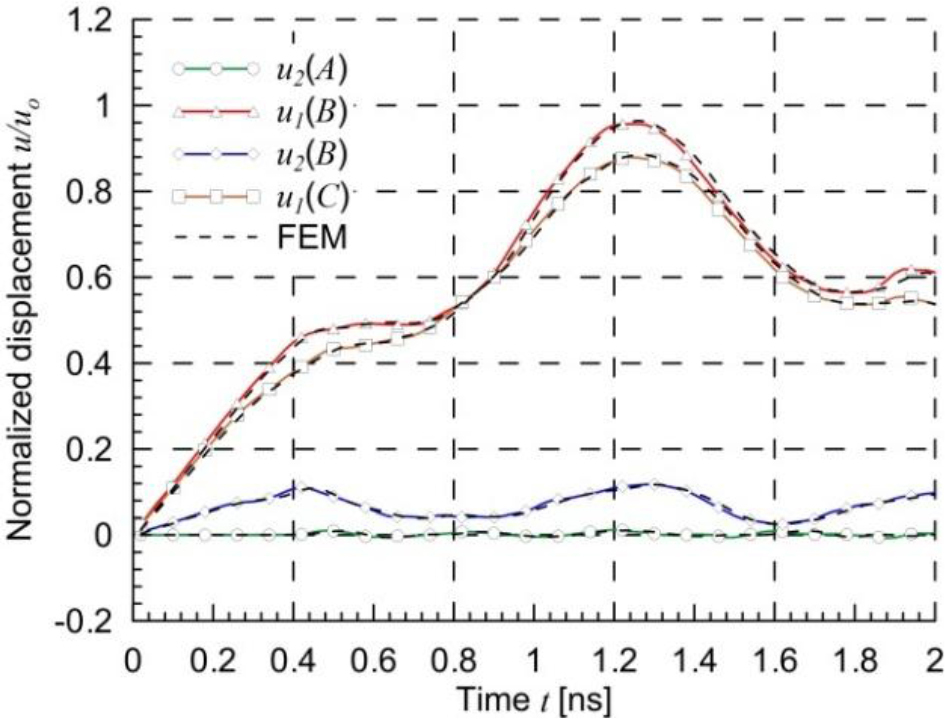
The displacements of points on the dynamically loaded edge of reinforced plate in both cases of boundary conditions are smaller than the displacements of a statically loaded matrix without a nanotube.

For a plate loaded along one edge, the influence of the number of boundary elements on the accuracy of the displacements of point C u₁ in the horizontal direction was investigated. The method of division into boundary elements is presented in Table 1. The results are presented in Fig. 9. On the basis of the calculations, it can be concluded that the method converges quickly. Since very good results were obtained for the third discretization method, and further increasing the number of boundary elements has little effect on the accuracy of displacements, the same division of the nanotube into elements and a similar length of elements for the external boundary will be used in subsequent examples.

Fig. 9.

Rectangular plate with a single nanotube – normalized displacements of point C for different number of boundary elements

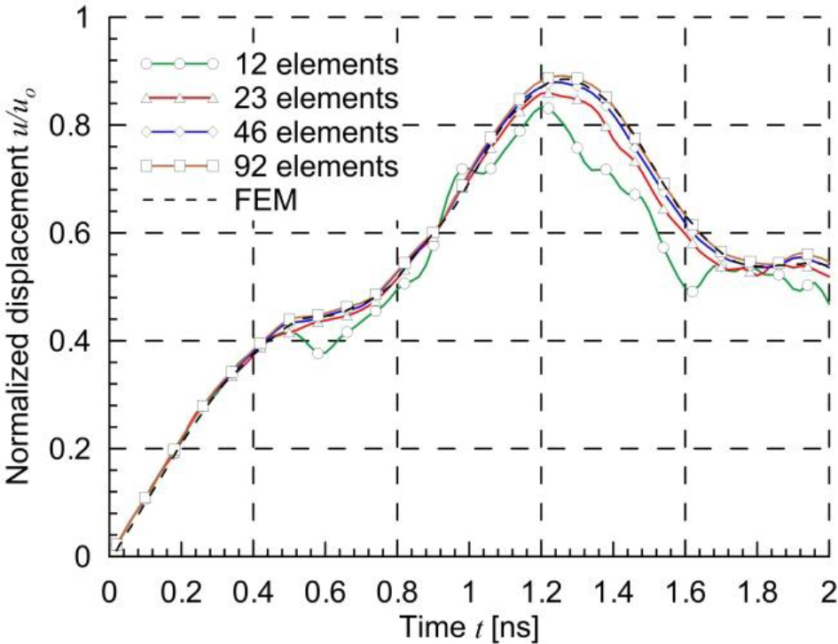
Tab. 1.

Division of the rectangular plate with a single nanotube into boundary elements

Discretization	Number of boundary elements
	nanotube	external boundary	total
1	2	10	12
2	5	18	23
3	10	36	46
4	20	72	92

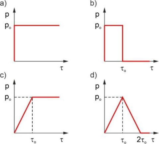
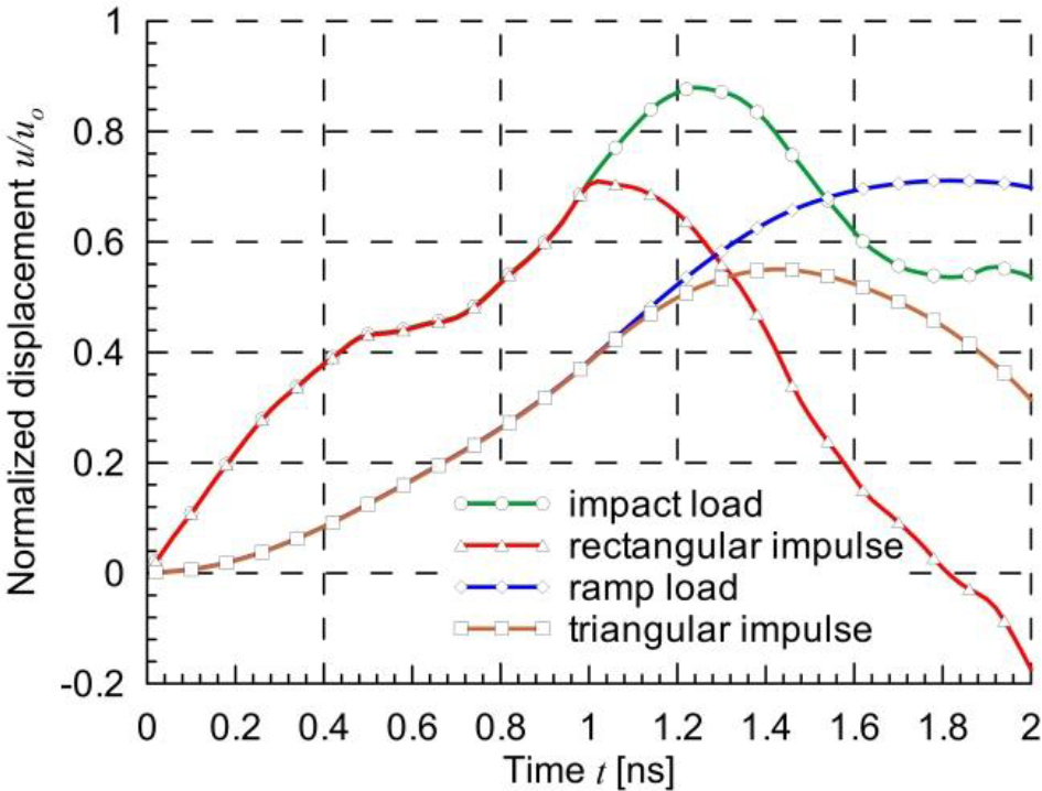
For the same example, the influence of load variability over time on the horizontal displacement of point C was examined. Four load cases were considered, as shown in Fig. 10: impact load, rectangular impulse, ramp load, and triangular impulse. The value p_o denotes the maximum load, and t_o denotes the characteristic time, which was assumed to be t_o=1 ns. The displacements are shown in Fig. 11. The plot presents the same displacements for the impact load and rectangular impulse, as well as for the ramp load and the triangular impulse, up to a time of t_o=1 ns, because the initial load variation up to this time is the same. The largest displacements are caused by the impact load, and this load will be considered in subsequent examples.

Fig. 10.

Load variability over time: a) impact load, b) rectangular impulse, c) ramp load, d) triangular impulse

Fig. 11.

Rectangular plate with a single nanotube - normalized displacements of point C for different variability of load over time

Rectangular plate with 15 nanotubes – influence of distance between nanotubes

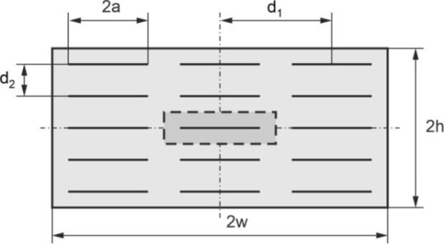
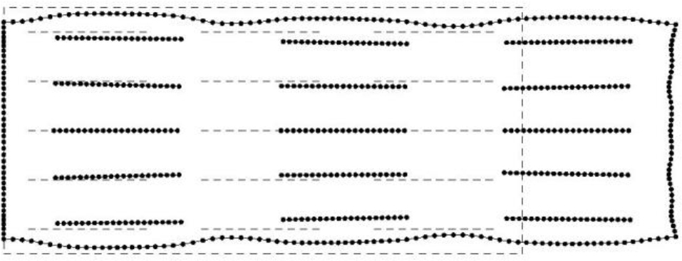
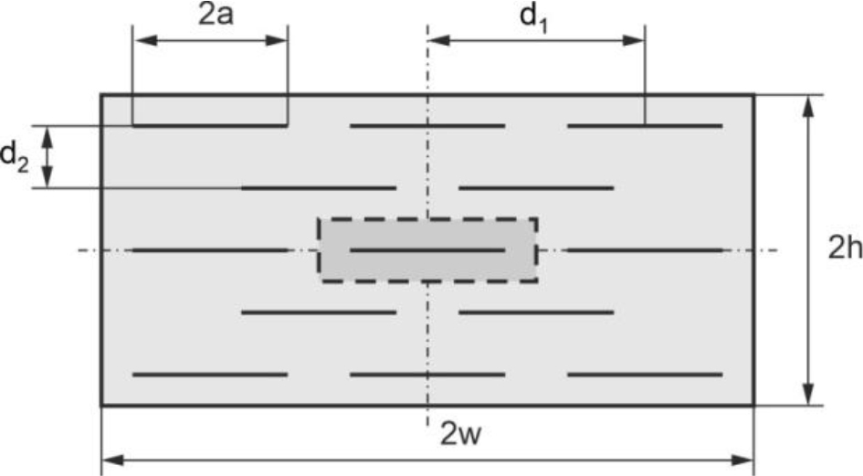
A rectangular plate of length 2w=4.2 μm and height 2h=2.0 μm contains 15 parallel nanotubes of length 2a=1.0 μm, as shown in Fig. 12. The horizontal distance between the centers of the nanotubes is d₁=1.4 μm and the vertical distance is d₂=0.4 μm. The area marked in grey denotes the part of the composite considered in the first example. The plate is divided into 270 boundary elements – 120 elements are used for the external boundary and 10 elements for each nanotube. In the FEM the whole plate is divided into 3360 four-node quadrilateral elements.

Fig. 12.

Rectangular plate with 15 nanotubes – dimensions of the plate

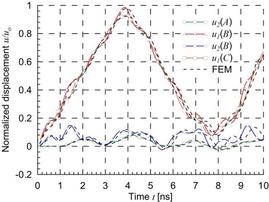
A comparison of normalized displacements of three selected points obtained by the BEM and FEM for two-edge and one-edge loadings is shown in Figs. 13 and 14, respectively. Very good agreement of the results obtained by the two methods can be seen. The initial and deformed shape of the plate, for one-edge loading, at time t=4 ns, when the displacements have large values (see Fig. 14) are shown in Fig. 15. Small deformations can be seen in the surroundings of nanotubes and large between them.

Fig. 13.

Rectangular plate with 15 nanotubes – normalized displacements of selected points for two-edge loading

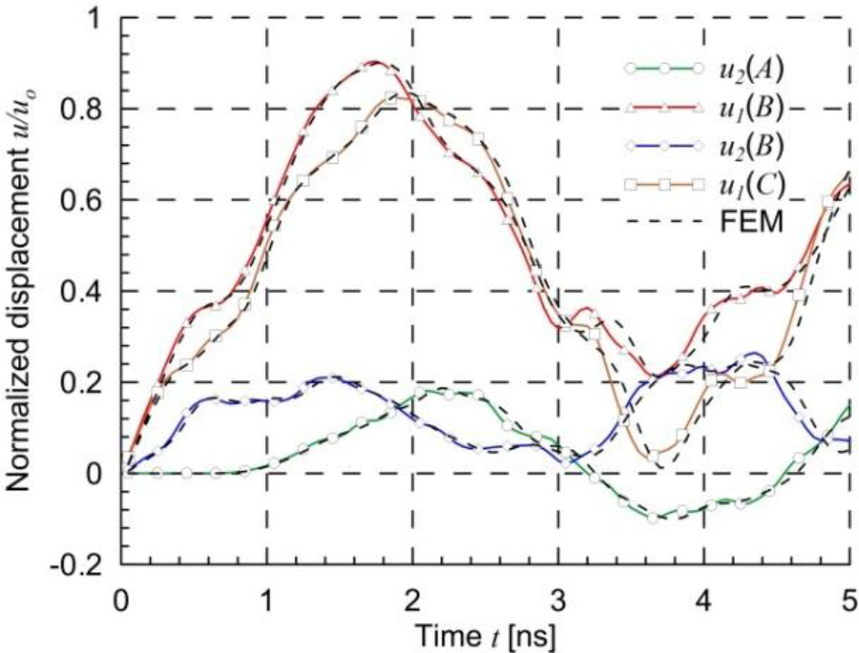
Fig. 14.

Rectangular plate with 15 nanotubes – normalized displacements of selected points for one-edge loading

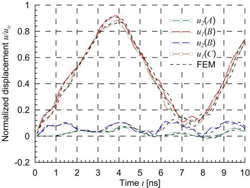
Fig. 15.

Rectangular plate with 15 nanotubes – initial and deformed shape of the plate at time t=4 ns for one-edge loading

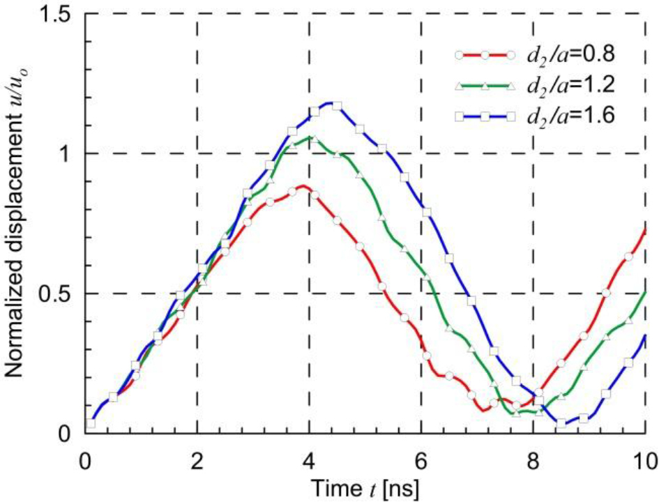
The influence of vertical distance between nanotubes on the displacement u₁ of point C in the horizontal direction for a one-edge loading is studied. Three different relative distances are considered d₂/a=0.8, 1.2 and 1.6. The case d₂/a=0.8 is the main case, which was analyzed in Fig. 14. The height of the plate is proportional to the distance between the nanotubes 2h=2.0, 3.0 and 4.0 μm and the length is constant 2w=4.2 μm. It can be seen in Fig. 16 that increasing the distance between the nanotubes by 100% from the value d₂/a=0.8 to the value 1.6 results in a 34% increase in the maximum displacement. The maximum displacement values for larger nanotube distances occur later.

Fig. 16.

Rectangular plate with 15 nanotubes – influence of the vertical distance between nanotubes on displacements

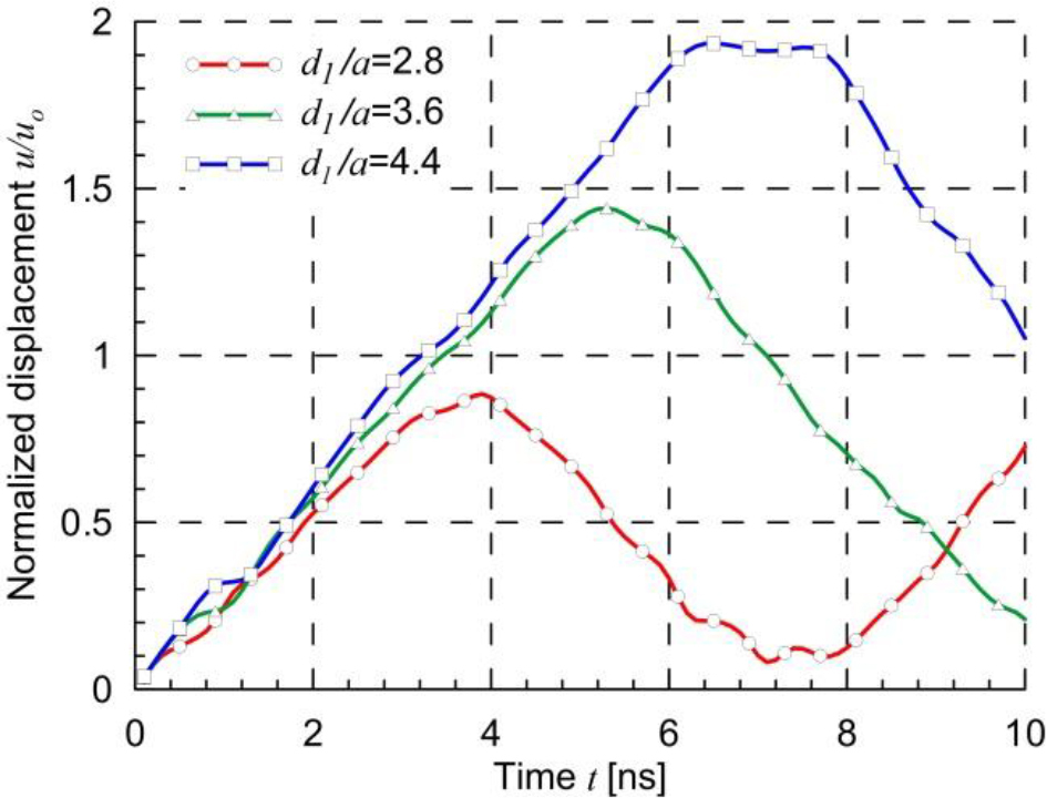
The influence of the horizontal distance between the nanotubes on the displacement u₁ of point C in the horizontal direction for one-edge loading is studied. Three different relative distances are considered d₁/a=2.8, 3.6 and 4.4. The case d₁/a=2.8 is the main case, which was analyzed in Fig. 14. The length of the plate is proportional to the distance between the nanotubes 2w=4.2, 5.4 and 6.6 μm and the height is constant 2h=2.0 μm.

It can be seen in Fig. 17 that increasing the distance between the nanotubes by 57% from the value d₁/a=2.8 to the value 4.4 results in a 218% increase in maximum displacement. The maximum displacement values for larger nanotube distances occur later.

An increase in the distance between the nanotubes in the nanotube direction has a greater effect on the displacement of the loaded edge than in the direction perpendicular to the nanotubes.

Fig. 17.

Rectangular plate with 15 nanotubes – influence of the horizontal distance between nanotubes on displacements

Rectangular plate with 13 nanotubes – influence of length of nanotubes

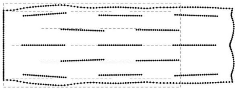
A rectangular plate contains 13 parallel nanotubes uniformly distributed, as shown in Fig. 18. The dimensions of the plate and distances between nanotubes are the same as in the previous main example 5.2. The plate is divided into 250 boundary elements – 120 elements are used for the external boundary and 10 elements for each nanotube. In the FEM the whole plate is divided into 3360 four-node quadrilateral elements.

Fig. 18.

Rectangular plate with 13 nanotubes – dimensions of the plate

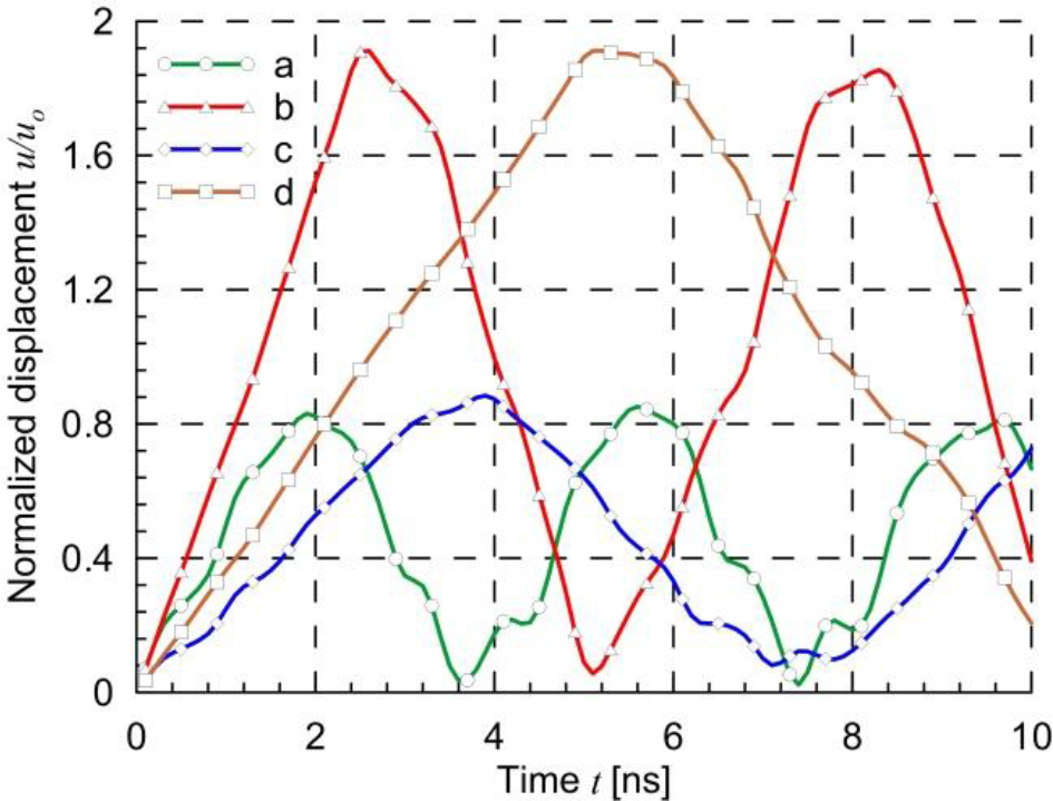
A comparison of normalized displacements of three selected points obtained by the BEM and FEM for two-edge and one-edge loading is shown in Figs. 19 and 20 respectively. Very good agreement of the results obtained by the two methods can be seen.

Fig. 19.

Rectangular plate with 13 nanotubes – normalized displacements of selected points for two-edge loading

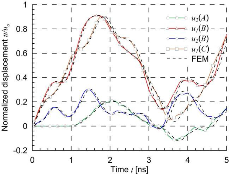
Fig. 20.

Rectangular plate with 13 nanotubes – normalized displacements of selected points for one-edge loading

The initial and deformed shape of the plate, for the one-edge loading, at time t=4 ns, when the displacements have large values (see Fig. 20) are shown in Fig. 21.

Fig. 21.

Rectangular plate with 13 nanotubes – initial and deformed shape of the plate at time t=4 ns for one-edge loading

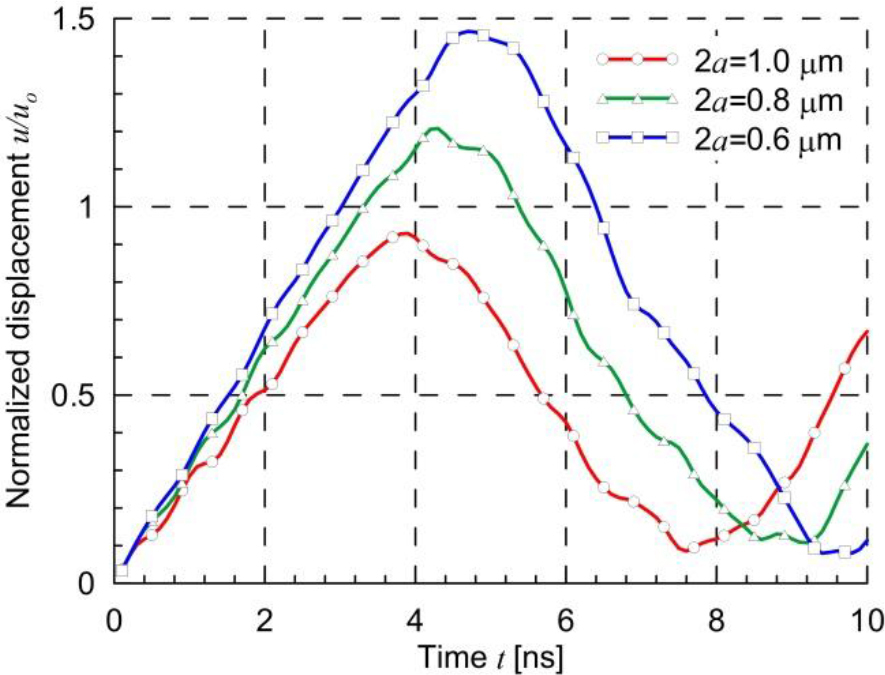
The influence of the length of the nanotubes on the displacement u₁ of point C in the horizontal direction for the one-edge loading is studied. Three different lengths of nanotubes are considered 2a=1.0, 0.8, and 0.6 μm. The case 2a=1.0 μm is the main case, which was analyzed in Fig. 20. The dimensions of the plate and the distances between the nanotubes are fixed and are the same as in the previous main example 5.3. It can be seen in Fig. 22 that decreasing the length of the nanotubes by 40% from the value 2a=1.0 μm to the value 0.6 μm results in a 58% increase in maximum displacement. The maximum displacement values for smaller nanotubes occur later.

Fig. 22.

Rectangular plate with 13 nanotubes – influence of the length of nanotubes on displacements

Analysis of the influence of reinforcement on the stiffness of nanocomposites

In order to investigate the effect of reinforcement on the stiffness of the nanocomposite, the displacements of point C were analyzed for the matrix alone and for the matrix with nanotubes. The longitudinal wave propagation velocity in the matrix is c₁=1834 m/s, and the shear wave velocity is c₂=981 m/s. Fig. 23 shows the displacements for the first example – a rectangular plate with a single nanotube, and Fig. 24 shows the displacements for the second example – a rectangular plate with 15 nanotubes. The conclusions from the calculations for both examples are similar.

Fig. 23.

Rectangular plate with a single nanotube – influence of reinforcement: a) with nanotube, two-edge loading, b) without nanotube, two-edge loading, c) with nanotube, one-edge loading, d) without nanotube, one-edge loading

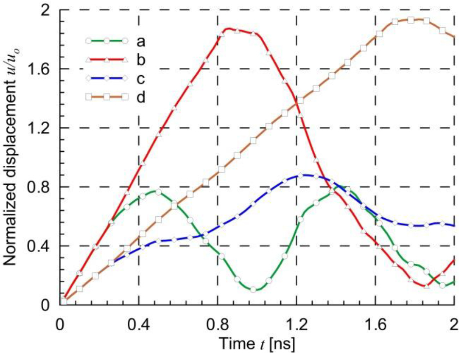
Fig. 24.

Rectangular plate with 15 nanotubes – influence of reinforcement: a) with nanotubes, two-edge loading, b) without nanotubes, two-edge loading, c) with nanotubes, one-edge loading, d) without nanotubes, one-edge loading

The maximum displacements of the dynamically loaded matrix alone are almost twice as large as the displacements for static loading. The use of reinforcement reduces the maximal displacements by more than twice. The displacements of the plate without reinforcement and with reinforcement are the same until approximately 0.3 ns, when the longitudinal wave propagates from the loaded edge to the nearest nanotube and returns after reflection to the edge. The displacements increase when the longitudinal wave propagates from the loaded edge to the vertical axis of symmetry for a two-edge loading or to the fixed edge in the case of a one-edge loading and returns back to the loaded edge. Therefore, the maximum displacements for a one-edge loading occur twice as late as for a two-edge loading. Because the reinforced composite has a higher stiffness than the matrix, the waves propagate faster in it, and the displacement changes occur more frequently than in the matrix alone.

5. CONCLUSIONS

The boundary element method is presented for analysis of dynamically loaded composites reinforced by carbon nanotubes. The nanotubes are treated as thin and perfectly rigid. Contrary to domain methods, the BEM allows analysis by discretization of external boundaries and nanotubes. Because only boundaries are discretized it is very easy to change the length of nanotubes and their distribution in nanocomposites. The present method can be used efficiently to study the influence of reinforcement on the displacements of nanocomposites. The accuracy of the computer code was investigated by comparing the displacements of the selected points with the FEM solutions.

The following conclusions can be deduced from the numerical calculations:

The following directions for further research can be considered: