Exploring Jacobi Elliptic and Periodic Solitary Wave Solutions for the Family of 3-D WBBM Equations Through the Generalized Approach

In this paper, we analyze the family of three-dimensional Wazwaz-Benjamin-Bona-Mahony (3-D WBBM) equations using the generalized Jacobi elliptic function expansion method. Understanding complicated wave patterns is critical, therefore, the family of 3-D WBBM equations is a valuable mathematical model with application in fluid mechanics, plasma dynamics, biomechanics, and engineering sciences. The main objective of this study is to build several new multiple wave form solutions for the nonlinear three-dimensional Wazwaz-Benjamin-Bona-Mahony (3-D WBBM) equations. By first using the travelling wave transformation, the nonlinear partial differential equation is transformed into an ordinary differential equation. Then the generalized Jacobi elliptic function expansion method is used to execute a finite series expansion of degree n. Due to this analytical method, we obtained numerous new exact solutions, including periodic solutions in Jacobi elliptic function forms and their corresponding Solitary and shock wave solutions in a limit convergence sense when the modulus parameter m approaches 1 and 0. These results are particularly useful for nonlinear science and mathematical physics professionals, since they provide important insights into the structure and evolution of nonlinear waves in a variety of physical circumstances. To improve the physical description of the solutions, several typical wave profiles are offered to provide a comprehensive analysis of the wave characteristics of the solutions in 2-D, 3-D, and contour visualizations were generated using accurate parameters value with the help of Mathematica. Moreover, by generating novel and accurate propagating soliton waveform solutions, the generalized Jacobi elliptic function expansion methods highlight its importance in uncovering key aspects of the model behaviours as well as suggesting potential applications in the study of water waves.

1. INTRODUCTION

Nonlinear phenomena occur in various scientific domains, including applied mathematics, physics, and engineering. Nonlinear evolution equations (NLEEs) are being explored in multiple nonlinear areas, such as nonlinear optics, thermal conductivity, fluid mechanics, optical fiber, electromagnetism, quantum theory, and shallow water wave propagation [1–3]. The research on soliton wave solutions of NLEEs is drawing interest. Because the majority of physical systems are nonlinear, researchers have been encouraged to investigate whether exact solutions exist for NLPDEs, specifically nonlinear evolution equations, or evolution equations (EEs).

Numerous numerical and analytical approaches have been developed to address nonlinear partial differential equations. The researchers prefer analytical approaches over numerical methods because they provide an extensive understanding of physical processes and precise insights into system dynamics. However, analytically solving nonlinear partial differential equations (NLPDEs) can be challenging. For this purpose, in recent decades, much development has been done; many reliable and efficient techniques have been presented to achieve the exact NLEE solutions. Like the exp-function approach [4, 5], (G’/G)-expansion technique [6, 7], F-expansion approach [8, 9], modified extended tanh-function technique [10, 11], the Hirota bilinear technique [12, 13], the extended rational sin-cos and sinh-cosh methods [14], the generalized sine-gordon expansion approach [15], the modified Kudryashov technique [16], Variational Iteration Method [17], Improved (G’/G)-Expansion technique [18, 19], Riccati-Bernoulli Sub ODE approach [20] Generalized Exponential Rational Function approach [21] and so on. These methods have been effectively established and provided to find a precise solution for NLPDEs. Although these approaches have made great progress, but they often fail when used to more complex models, such as a family of 3-D WBBM equations, where more efficient and extended methodologies are needed.

This article uses an efficient and effective strategy to generate different types of periodic and solitary wave solutions for the three-dimensional WBBM equations. The three-dimensional WBBM equation can be stated as follows:

1.1

vx+v2vy+vt−vxzt=0,

1.2

vy+v2vx+vt−vxyt=0,

1.3

vz+v2vz+vt−vxxt=0.

Wazwaz proposed the 3-D Wazwaz-Benjamin-Bona-Mahony (3-D WBBM) equation in 2017 [22]. The 3-D WBBM equation is the modified form of the famous KdV equation, which is used to study the stability and soliton-like properties of fluid waves in various scientific phenomena. The family of Wazwaz-Benjamin-Bona-Mahony (3-D WBBM) equations has attracted much attention because of their mathematical structure and practical applications. This equation is characterized by a scenario that addresses nonlinearity and dispersion, making it valuable for analyzing wave phenomena in a physical setting. In recent years, several successful techniques have been applied to study the WBBM model, such as the first integral method [23], the modified Exp-function approach [24], the Generalized rational exponential function approach for analytical solutions [25], Rational sine-Gordon expansion approach [26], the Sardar-Sub equation approach [27], the Improved Bernoulli Sub-Equation Function technique [28], the extended modified auxiliary equation mapping (EMAEM) approach [29], a new extended direct algebraic technique [30], the ϕ6 expansion approach and modified extended direct algebraic [31], the Khater methods [32], and the expanded tanh approach [33]. In addition to the existing analytical methods, the generalized Jacobi elliptic function expansion method, previously applied to various nonlinear PDEs and FPDEs [34–42], has not yet been employed for the 3D WBBM model, offering potential for innovative exact solutions.

In this paper, we integrate the generalized Jacobi elliptic function expansion technique for studying the family of 3-D WBBM equations. The generalized JEFE method is more efficient and generalized than the existing methods for solving the 3-D WBBM equations. The generalized JEFE approach makes good use of Jacobi elliptic functions, allowing for a large number of solutions, such as Jacobian elliptic, trigonometric, and hyperbolic trigonometric functions type of solutions, which improves its application to diverse nonlinear wave equations. Furthermore, it is a noteworthy invention that constitutes notable progress. When solving nonlinear partial differential equations (PDEs), the generalized Jacobi elliptic function expansion technique has several advantages and disadvantages. Its ability to provide periodic and exact solutions is one of its primary features. In order to understand complicated nonlinear dynamics, this capacity is crucial. Equations exhibiting specific symmetries and invariants benefit greatly from this method, as it allows for a more thorough examination of the solutions. Its limited application, however, is one of its main drawbacks. The exact solutions demonstrated that our suggested WBBM equations are perfectly suitable for producing innovative traveling wave structures in a wide range of physical scenarios without any problems, in addition, the article contains details 2-D, contour, and 3-D graphical visualizations of the solutions to demonstrate how well the suggested method solves difficult nonlinear equations and to help readers better understand their physical features, to providing useful information for further research in mathematical physics and shallow water waves.

The following is the order of the work in this paper. Section 2 explains how to solve NLPDEs using generalized JEFE techniques. In Section 3, we describe how this approach can be used to solve the nonlinear 3-D WBBM system. This section is divided into three subsections, each of which presents Periodic wave solutions in terms of Jacobi elliptic function expansion, and solitary and shock wave solutions. Section 4 presents a graphical presentation and discussion. Section 5 presents the conclusion of the study.

2. SUMMARY OF THE GENERALIZED JEFE APPROACH

Within this part of the article, we explain the details of the generalized JEFE approach. The following steps will be followed when conducting these types of studies:

Step A: Nonlinear partial differential equations (NPDEs) typically take the mathematical expression
2.1
N(v,∂v∂t,∂v∂x,∂v∂z,∂2u∂x∂x,∂2u∂x∂t,∂2u∂x∂z,∂2u∂t∂t,…)=0.
Step B: Reformulating Equation (2.1) and utilizing the chain rule, we consider:
2.2
v(x,y,z,t)=v(ψ),where ψ=px+qy+rz−st,
where p,q,r, and represent constants. We can use equation (2.2) to convert the nonlinear PDEs (2.1) into ordinary differential equations.

2.3

N(v,∂v∂ψ,∂2v∂ψ2,…)=0.

The primary objective of this extended indirect strategy is to maximize the possibility of addressing the derived ordinary differential equation, more especially the initial kind of Jacobian problem that involves three variables, such as m₂, m₁, and m₀. The goal is to come up with a more comprehensive collection of Jacobi elliptic solutions for the problem that has been presented. It is possible to visually represent the auxiliary equation as follows:

2.4

(N′)2(ψ)=m2N4(ψ)+m1N2(ψ)+m0,

where

N′=dNdψ, ψ=ψ(x,y,z,t), and ,m2, m1, and m0

are constants.

The mathematical expressions for Jacobi elliptic functions are given by:

sn(ψ)= sn(ψ, k), cn(ψ)= cn(ψ, k), dn(ψ)= dn(ψ, k)

Here, the k is used to signify the modulus, and k ∈ (0,1).

The solutions of equation (2.4) are presented in Tab.1.

Tab. 1.

The following table summarizes all the potential solutions to equation (2.3) for the specific m₂, m₁, and m₀ values that have been provided

NO.	m₂	m₁	m₀	N
1	k²	–(1 + k²)	1	sn
2	k²	–(1 + k²)	1	cd
3	–k²	2k² – 1	1 – k²	cn
4	–1	2 – k²	k² – 1	dn
5	1	–(1 + k²)	k²	ns
6	1	–(1 + k²)	k²	dc
7	1 – k²	2k² – 1	–k²	nc
8	k² – 1	2 – k²	–1	nd
9	1 – k²	2 – k²	1	sc
10	–k²(1 – k²)	2k² – 1	1	sd
11	1	2 – k²	1 – k²	cs
12	1	2k² – 1	-k²(1 – k²)	ds
13	−14	k2+12	−(1−k2)24	kcn ∓ dn
14	14	−2k2+12	14	ns ∓ cs
15	1−k24	k2+12	1−k24	nc ∓ sc
16	14	k2−22	k44	ns ∓ ds
17	k24	k2−22	k24	sc ∓ icn
18	k24	k2−22	k24	sn1−k2sn∓cn
19	k24	k2−22	k24	kcn ∓ idn
20	14	1−2k22	14	sn1∓cn
21	k24	k2−22	14	sn1∓dn
22	k2−14	k2+12	k2−14	dn1∓ksn
23	1−k24	k2+12	−k2+14	cn1∓sn
24	(1−k2)24	k2+12	14	sndn∓cn
25	k44	k2−22	14	cn1−k2∓dn

As k → 0 and k → 1, Jacobi elliptic functions, as mentioned in Table. simplify into periodic, trigonometric, and hyperbolic functions. Consequently, soliton solutions and solutions involving trigonometric functions are obtained for the problem. Using the application of the generalized Jacobi elliptic function expansion generalized JEFE technique, v(ψ) is formulated as a finite series of Jacobi elliptic functions

2.5

v(ψ)=∑i=0naiNi(ψ), i=0,1,2,…n.

Where N(ψ) provides the solution to the nonlinear ODE (2.4) with a_i being constants that will be determined subsequently.

The integer n can be derived from equation (2.5) by considering the maximum order derivative component:

2.6

O(dαvdψα)=n+α, α=0,1,2,3,…

and the nonlinear component with the highest power of the differential equation

2.7

O(vβdαvdψα)=(β+1)n+α,β=1,2,3,

in equation (2.3).

Using equation (2.5) and setting all the coefficients corresponding to powers of N equal to 0, we establish a series of nonlinear algebraic equations corresponding to the coefficient a_i of equation (2.5) Utilising Maple, we resolve this system and substitute all the parameters for m₂,m₁ from equation (2.4) into Table 1. This approach integrates the value of equation (2.5) with the selected auxiliary equation, allowing for the derivation of accurate solutions for equation (2.1).

3. MATHEMATICAL FORMULATION OF THE GENEERALIZED JEFE APPROACH

Analysis of the first WBBM equation

Let the first three-dimensional WBBM equation be expressed as:

3.1

∂tu+∂xu+∂yu3−∂xzt3u=0,

where ∂ represents partial derivative. Utilizing the wave transformation:

3.2

v(x,y,z,t)=v(ψ),

where

ψ=p x + q y + r z − s t,

and substituting into Eq. (3.2) we obtain:

3.3

(−c + p)v′+ q(v3)′+ prcv′′′= 0.

Integrating Equation (3.3) w.r.t ψ yields:

3.4

(−c + p)v + qv3+ prcv′′+ C = 0.

Here, the C acts as the arbitrary constant arising from integration. For simplicity, setting C = 0, we have:

3.5

(−c + p)v + qv3+ prcv′′= 0.

Considering the homogeneous balancing of the derivative component of maximum order v″ and the nonlinear component v³ in Eq. (3.5), it is clear that n = 1. Thus, the method suggests the following supplementary solution:

3.6

v(ψ)=b0+ b1N(ψ).

Differentiating Eq. (3.6) with respect to ψ, we have:

3.7

v′(ψ)=b1′N′(ψ).

Substituting this into the governing equation, we get:

3.8

v′(ψ)=b1(m2N4(ψ)+m1N2(ψ)+m0)12v′′(ψ)=b1N(ψ)(2m2N2(ψ)+m1).

Substitute Eq. (3.8) and Eq. (3.7) into the equation

3.9

−s b0− sb1N(ψ)+ pb0+ pb1N(ψ)+qb03+3qb02b1N(ψ)+3qb0b12N(ψ)2+qb13N(ψ)3+prs b1N(ψ)m0+2prs b1N(ψ)m2=0.

By collecting various powers of Nⁱ(ψ), a subsequent set of algebraic equations is derived:

3.10

−s b0+p b0+q b03=0,

3.11

−s b1+p b1+3 q b02b1+p r s b1m1= 0,

3.12

3 q b0b12=0,

3.13

q b13+ 2p r s b1m2= 0.

The system described above of algebraic equations is calculated through MAPLE, and we derive the roots of the coefficients involved in equation (3.6):

3.14

b0 = 0,

3.15

b1=±2r m2−q+q p r m1p,

3.16

S=p1−pr m1.

The following solutions for the 3-D WBBM equation can be obtained by inserting the corresponding values into Eq. (3.6):

3.17

v(x,y,z,t)=±2r m2−q+q p r m1p N( p x + q y + r z −p1−pr m1t).

Analytical periodic solutions in terms of Jacobi elliptic functions (JEF)

Using the data provided in Table 1 and Table 2 and combining the corresponding values as per Eq. (3.6), we may derive the Jacobi elliptic function solutions which are of a periodic nature for Eq. (1.1) as shown below.

3.18

v1,1(x,y,z,t)=±−2k2r(pr(k2+1)+q)psn(px+qy+rz−pt1+pr(k2+1)),

3.19

v1,2(x,y,z,t)=±−2k2r(pr(k2+1)+q)pcd(px + qy + rz −pt1+pr(k2+1)),

3.20

v1,3(x,y,z,t)=±−2k2r(pr(2k2−1)+q)pcn(px + qy + rz −ptpr(2k2−1)+1),

3.21

v1,4(x,y,z,t)=±2r(pr(1−k2)+q)pdn(px + qy + rz −ptpr(2−k2)+1),

3.22

v1,5(x,y,z,t)=±−2r(q−pr(k2+1))pns(px + qy + rz −pt1−pr(k2+1)),

3.23

v1,6(x,y,z,t)=±−2rq(pr(k2+1)+1)pdc(px + qy + rz −ptpr(−k2−1)+1),

3.24

v1,7(x,y,z,t)=±−2r(k2−1)q(pr(2k2−1)−1)pnc(px + qy + rz −ptpr(2k2−1)+1),

3.25

v1,8(x,y,z,t)=±−2r(k2−1)(prq(2k2−2)+q)pnd(px + qy + rz −ptpr(2−k2)+1),

3.26

v1,9(x,y,z,t)=±2r(k2−1)(prq(k2−2)+q)psc(px + qy + rz −ptpr(2−k2)+1),

3.27

v1,10(x,y,z,t)=±2k2r(k2−1)(prq(2k2−1)−q)psd(px + qy + rz−ptpr(2k2−1)+1),

3.28

v1,11(x,y,z,t)=±−2r(q(pr(k2−2)+1))pcs(px + qy + rz −ptpr(2−k2)+1),

3.29

v1,12(x,y,z,t)=±2r(prq(2k2−1)−q))pds(px +qy+rz−ptpr(2k2−1)+1),

3.30

v1,13(x,y,z,t)=±−r(q(pr(k2+1)−2))p [kcn(px + qy + rz −ptpr(k2+1)2+1)± dn(px + qy + rz −ptpr(k2+1)2+1)],

3.31

v1,14(x,y,z,t)=±−r(q(pr(1−2k2)−2))p[ns(px+qy+rz−pt1−pr(1−2k2)2)±cs(x+qy+rz−pt1−pr(1−2k2)2)p],

3.32

v1,15(x,y,z,t)=±−r(k2−1)(q(pr(k2+1)−2))· p [nc(px + qy + rz − pt(1−pr(k2+1)2))±sc (px + qy + rz − pt(1−pr(k2+1)2))],

3.33

v1,16(x,y,z,t)=±r(prq(k2−2)−2q)p [ns(px + qy + rz − pt(1−pr(k2−2)2))± ds (px + qy + rz − pt(1−pr(k2−2)2))],

3.34

v1,17(x,y,z,t)=±k2r(q(pr(k2−2)−2))p [sn(px + qy + rz − pt(1−pr(k2−2)2))±icn(px + qy + rz − pt(1−pr(k2−2)2))],

3.35

v1,18(x,y,z,t)=±k2r(q(pr(k2−2)−2))psn(px + qy + rz −pt(1−pr(k2−2)2))(1−k2)±cn(px+qy+rz−pt(1−pr(k2−2)2)),

3.36

v1,19(x,y,z,t)=±k2r(pqr(2k2−2)+2q)p [kcn(px + qy + rz −pt(1−pr(1−2k2)2))±idn(px + qy + rz −pt(1−pr(1−2k2)2))],

3.37

v1,20(x,y,z,t)=±−r(prq(1−2k2)+2q)psn(px + qy + rz −pt(1−pr(1−2k2)2))1±cn(px + qy + rz −pt(1−pr(1−2k2)2)),

3.38

v1,21(x,y,z,t)=±k2r(pqr(k2−2)−2q)psn(px + qy + rz −pt(1−pr(k2−2)2))(1−k2)±d n(px + qy + rz −pt(1−pr(k2−2)2)),

3.39

v1,22(x,y,z,t)=±r(k2−1)q(pr(k2+1)−2)pdn(px + qy + rz −pt(1−pr(k2+1)2))1±ksn(px + qy + rz −pt(1−pr(k2+1)2)),

3.40

v1,23(x,y,z,t)=±−(rk2−r)(pqr(k2+1)−2q)pcn(px+qy+rz−pt(1−pr(k2+1)2))1±sn(px+qy+rz−pt(1−pr(k2+1)2)),

3.41

v1,24(x,y,z,t)=±−r(k2−1)2(pqr(k2+1)−2q)psn(px + qy + rz −pt(1−pr(k2+1)2))dn(px + qy + rz−pt(1−pr(k2+1)2))±cn(px + qy + rz −pt(1pr(k2+1)2)),

3.42

v1,25(x,y,z,t)=±k4r(q(pr(k2−2)−2))pcn(px + qy + rz −pt(1−pr(k2−2)2))(1−k2)±dn(px + qy + rz −pt(1−pr(k2−2)2)).

Tab. 2.

The Jacobi elliptic function exhibit specific limiting behaviour as k → 0 and k → 1

No.	Function	k → 1	k → 0
1	sn(v)	tanh(v)	sin(v)
2	cn(v)	sech(v)	cos(v)
3	dn(v)	sech(v)	1
4	cd(v)	1	cos(v)
5	sd(v)	sinh(v)	sin(v)
6	nd(v)	cosh(v)	1
7	dc(v)	1	sec(v)
8	nc(v)	cosh(v)	sec(v)
9	sc(v)	sinh(v)	tan(v)
10	ns(v)	coth(v)	csc(v)
11	ds(v)	csch(v)	csc(v)
12	cs(v)	csch(v)	ct(v)

Solitary wave solutions

When k → 1, in this category, see in table 2, the solutions v_1,7, v_1,8, v_1,9, v_1,10, v_1,15, v_1,22, v_1,23 and v_1,24 become zero. The remaining solutions represent solitary wave solutions and can be determined as follows:

3.43

v1,26(x,y,z,t)=±−2r(2prq+q)p tanh(px + qy + rz −pt2pr+1),

3.44

v1,27(x,y,z,t)=±−2r(prq−q)p sech(px + qy + rz −ptpr+1),

3.45

v1,28(x,y,z,t)=±2r(−prq+q)p sech(px + qy + rz −ptpr+1),

3.46

v1,29(x,y,z,t)=±−2r(2prq+q)p coth(px + qy + rz −pt−2pr+1),

3.47

v1,30(x,y,z,t)=±−2r(−prq+q)p csch(px + qy + rz −pt−pr+1),

3.48

v1,31(x,y,z,t)=±r(prq−q)p csch(px + qy + rz −ptpr+1),

3.49

v1,32(x,y,z,t)=±−r(2prq−2q)p [sech(px + qy + rz −ptpr+1)±sech(px + qy + rz −ptpr+1)],

3.50

v1,33(x,y,z,t)=±r(prq+2q)p [coth(px + qy + rZ −pt12pr+1)±csch (px + qy + rz −pt12pr+1)],

3.51

v1,34(x,y,z,t)=±r(−prq−2q)p [coth(px + qy + rz −pt1+12pr)±csch(px + qy + rz −pt1+12pr)],

3.52

v1,35(x,y,z,t)=±r(−prq−2q)p [tanh(px + qy + rz −pt1+12pr)±isech(px + qy + rz −pt1+12pr)],

3.53

v1,36(x,y,z,t)=±r(−prq−2q)ptanh(px + qy + rz −pt1+12pr)sech(px + qy + rz −pt1+12pr),

3.54

v1,37(x,y,z,t)=±−r(prq+2q)p [sech(px + qy + rz −pt1+12pr)±isech(px + qy + rz −pt1+12pr)],

3.55

v1,38(x,y,z,t)=±−r(−prq+2q)ptanh(px + qy + rz −pt1+12pr)1±sech(px + qy + rz−pt1+12pr),

3.56

v1,39(x,y,z,t)=±−r(−prq−2q)ptanh(px + qy + rz −pt1+12pr)1±sech(px + qy + rz −pt1+12pr),

3.57

v1,40(x,y,z,t)=±r(−prq−2q)psech(px+qy+rz−pt1−12pr)sech(px+qy+rz−pt1−12pr).

Shock wave solutions

When k → 0, in this category see in table 2, the solutions v_1,2, v_1,3, v_1,10, v_1,17, v_1,18, v_1,21, and v_1,25 become Zero. The remaining solutions represent solitary wave solutions and can be determined as follows:

3.58

v1,41(x,y,z,t)=±−2r(prq+q)p csc(px + qy + rz −pt−pr+1),

3.59

v1,42(x,y,z,t)=±−2r(prq+q)p sec(px + qy + rz −pt−pr+1),

3.60

v1,43(x,y,z,t)=±−2r(prq+q)p sec(px + qy + rz −pt−nr+1),

3.61

v1,44(x,y,z,t)=±r(2prq−q)p tan(px+qy+rz−pt2pr+1),

3.62

v1,45(x,y,z,t)=±2r(2prq−q)p cot(px + qy + rz −pt2pr+1),

3.63

v1,46(x,y,z,t)=±−2r(prq+q)p csc(px + qy + rz −pt−pr+1),

3.64

v1,47(x,y,z,t)=±−r(prq−2q)p [csc(px + qy + rz −pt1−12pr)±cot(px + qy + rz −pt1−12pr)],

3.65

v1,48(x,y,z,t)=±−r(prq−2q)p [sec(px + qy + rz −pt1−12pr)±tan(px + qy + rz−pt1−12pr)],

3.66

v1,49(x,y,z,t)=±−2r(prq+2q)p [csc(px + qy + rz −pt1+pr)±csc(px + qy + rz −pt1+pr)],

3.67

v1,50(x,y,z,t)=±r(prq-2q)psin(px + qy + rz -pt1-12pr)1±cos(px + qy + rz -pt1-12pr),

3.68

v1,51(x,y,z,t)=±r(prq−2q)pcos(px + qy + rz −pt1−12pr)1±sin(px + qy + rz −pt1−12pr),

3.69

v1,52(x,y,z,t)=±r(prq−2q)psin(px + qy + rz −pt1−12pr)1±cos(px + qy + rz −pt1−12pr),

Analysis of the Second WBBM Equation

Using the traveling wave transformation equation (3.2) into equation (1.2), we convert the nonlinear partial differential equation (PDE) to an ordinary differential equation (ODE) of the following form:

3.70

(−s+r)v′+pv3+pqsv′′=0.

By the balancing procedure, we find the value of n = 1. Thus, the ansatz solution has the following simplified form:

3.71

v(ψ)=c0+c1N(ψ).

Substituting equation (3.71) combine with equation (2.4) into (3.70), we get:

3.72

−sc0− sc1N(ψ)+pc0+pc1N(ψ)+qc03+3q c02 c1N(ψ)+ 3q c0c12N(ψ)2+ qc13N(ψ)3+p r s c1N(ψ)m0+ 2p r s c1N(ψ)m2= 0.

By collecting various powers of Nⁱ(ψ), a subsequent system of algebraic equations is derived:

3.73

−sc0 + pc0 + qc0= 0,

3.74

−sc1 + pc1 +3qc0c1+prsc1 m1 = 0,

3.75

3qc0c12= 0,

3.76

qc13 + 2prs c1m2 = 0.

The system described above of algebraic equations is calculated through MAPLE, and we derive the roots of the coefficients involved in equation (3.71):

3.77

c0= 0,

3.78

c1= ±2qr m2−1 + p q m1,

3.79

S=r1− p q m1.

The following solutions for the first 3-D WBBM equation can be obtained by inserting the corresponding values into Eq. (3.71):

3.80

vx,y,z,t= ±2qr m2−1 + p q m1 p N ( px + qy + rz − 2qr m2−1+ p q m1).

Analytical periodic solutions in terms of Jacobi elliptic functions (JEF)

Using the data provided in Tables 1 and 2, and combining the corresponding values as per Eq.(3.71), we may derive the Jacobi elliptic function solutions which are periodic for equation (1.3) as shown below.

3.81

v2,1(x,y,z,t)=± 2qr k2−1−pq(k2+1)p sn (px + qy +rz−r1+pq(k2+1)t),

3.82

v2,2(x,y,z,t)=±|2qr k2−1−p q(k2 + 1)p cd(px + qy +rz−r1+pq(k2+1)t),

3.83

v2,3(x,y,z,t)=±−2k2qr(pq(2k2−1)−1)pcn(px+qy+rz−r(1−pq(2k2−1))t),

3.84

v2,4(x,y,z,t)=±−2qr(pq(2−k2)−1)pdn(px+qy+rz−r(1−pq(2−k2))t),

3.85

v2,5(x,y,z,t)=±2qr(−pq(k2+1)−1)pns(px+qy+rz−r(1+pq(k2+1))t),

3.86

v2,6(x,y,z,t)=±2qr(−pq(k2+1)−1)pdc(px+qy+rz−r(1+pq(k2+1))t),

3.87

v2,7(x,y,z,t)=±−2qr(k2−1)(pq(2k2−1)−1)pnc(px+qy+rz−rt(1−pq(2k2−1))),

3.88

v2,8(x,y,z,t)=±−2qr(k2−1)(pq(k2−2)+1)p nd(px+qy+rz−r(1−pq(2−k2))t),

3.89

v2,9(x,y,z,t)=±−2qr(k2−1)(pq(k2−2)+1)p sc(px+qy+rz−r(1−pq(2−k2))t),

3.90

v2,10(x,y,z,t)=±−2qr(k2−1)(pq(2k2−1)−1)p sd(px+qy+rz−r(1−pq(2k2−1))t),

3.91

v2,11(x,y,z,t)=±2qr(pq(2−k2)−1)p cs(px+qy+rz−r(1−pq(2−k2))t),

3.92

v2,12(x,y,z,t)=±2qr(pq(2k2−1)−1)p ds(px+qy+rz−r(1−pq(2k2−1))t),

3.93

v2,13(x,y,z,t)=±−qr(pq(k2+1)−2)p[kcn(px+qy+)rz−r(1−pq(k2+1)2)t±dn(px+qy+rz−r(1−pq(k2+1)2)t)],

3.94

v2,14(x,y,z,t)=±qr(pq(−2k2+1)−2)p[ns(px+qy+rz−r(1−pq(−2k2+1)2)t)±cs(px+qy+rz−r(1−pq(−2k2+1)2)t)],

3.95

v2,15(x,y,z,t)=±(−qr(k2−1))(pq(k2+1)−2)p[nc(px+qy+rz−r(1−pq(k2+1)2)t)±sc(px+qy+rz−r(1−pq(k2+1)2t)t)],

3.96

v2,16(x,y,z,t)=±qr(pq(k2−2)−2)p[ns(px+qy+rz−r(1−pq(k2−2)2)t)±ds(px+qy+rz−r(1−pq(k2−2)2)t)],

3.97

v2,17(x,y,z,t)=±k2qr(pq(k2−2)−2)p[sn(px+qy+rz−r(1−pq(k2−2)2)t)±icn(px+qy+rz−r(1−pq(k2−2)2)t)],

3.98

v2,18(x,y,z,t)=±k2qr(pq(k2−2)−2)psn(px+qy+rz−pt(1−pq(k2−2)2))((1−k2)±cn(px+qy+rz−pt(1−pq(k2−2)2)),

3.99

v2,19(x,y,z,t)=±−qr(pq(2k2−1)+2)p[kcn(px+qy+rz−r(1−pq(1−2k2)2)t)±idn(px+qy+rz−r(1−pq(1−2k2)2t)t),

3.100

v2,20(x,y,z,t)=±−qr(pq(2k2−1)+2)psn(px+qy+rz−pt(1−pq(1−2k2)2))1±cn(px+qy+rz−pt(1−pq(1−2k2)2)),

3.101

v2,21(x,y,z,t)=±−k2qr(pq(k2−2)−2)psn(px+qy+rz−pt(1−pq(k2−2)2))1±dn(px+qy+rz−pt(1−pq(k2−2)2)),

3.102

v2,22(x,y,z,t)=±qr(k2−2)(pq(k2+1)−2)pdn(px+qy+rz−pt(1−pq(k2+1)2))1±ksn(px+qy+rz−pt(1−pq(k2+1)2)),

3.103

v2,23(x,y,z,t)=±−qr(k2−2)(pq(k2+1)−2)pcn(px+qy+rz−pt(1−pq(k2+1)2))1±sn(px+qy+rz−pt(1−pq(k2+1)2)),

3.104

v2,24(x,y,z,t)=±qr(k2−2)2(pq(k2+1)−2)psn(px+qy+rz−pt(1−pq(k2+1)2))dn(px+qy+rz−pt(1−pq(k2+1)2))±cn(px+qy+rz−pt(1−pq(k2+1)2)),

3.105

v2,25(x,y,z,t)=±−k4qr(pq(k2−2)−2)pcn(px+qy+rz−pt(1−pq(k2−2)2))((1−k2)±dn(px+qy+rz−pt(1−pq(k2−2)2)),

Solitary wave type solutions

When k → 1, in this category see in table 2, the solution v_2,7, v_2,8, v_2,9, v_2,10, v_2,15, v_2,22, v_2,23 and v_2,24 become zero. The remaining solutions represent solitary wave solutions and can be determined as follows:

3.106

v2,26(x,y,z,t)=±2qr−1−2pqp tanh(px+qy+rz−r1+2pqt),

3.107

v2,27(x,y,z,t)=±−2qrpq−1p sech(px+qy+rz−r1−pqt),

3.108

v2,28(x,y,z,t)=±−2qrpq−1p sech(px+qy+rz−r1−pqt),

3.109

v2,29(x,y,z,t)=±2qr−2pq−1p coth(px+qy+rz−r1+2pqt),

3.110

v2,30(x,y,z,t)=±−2qrpq+1p csch(px+qy+rz−r1+pqt),

3.111

v2,31(x,y,z,t)=±2qr−pq−1p csch(px+qy+rz−r1+pqt),

3.112

v2,32(x,y,z,t)=± −2qr2pq−2p [sech(px + qy +rz − r1−pqt) ± sech (px + qy + rz − r1−pqt)],

3.113

v2,33 (x,y,z,t)=± qr−pq−2p [coth (px + qy + rz − r1+12pqt) ± csch (px + qy + rz − r1+12pqt)],

3.114

v2,34 (x,y,z,t)=± qr−pq−2p [coth(px + qy + rz + r−1−12pqt) ±csch (px + qy + rz + r−1−12pqt)],

3.115

v2,35 (x,y,z,t)=± qrpq−2p [tanh (px + qy + rz + r−1−12pqt) ± csch (px + qy + rz + r−1−12pqt)],

3.116

v2,36(x, y, z, t) =± qr−pq−2p tanh(px + qy + rz + r−1−12pqt)sech(px + qy + rz + r−1−12pqt),

3.117

v2,37(x,y,z,t)=±−qrpq+2p [sech (px + qy + rz + r−1−12pqt) ± isech (px + qy + rz + r−1−12pqt)],

3.118

v2,38(x,y,z,t)=±qrpq+2ptanh(px+qy+rz+r−1−12pqt)1±sech(px+qy+rz+r−1−12pqt),

3.119

v2,39(x,y,z,t)=±qr−pq−2ptanh(px+qy+rz+r−1−12pqt)1±sech(px+qy+rz+r−1−12pqt),

3.120

v2,40(x,y,z,t)=±qr−pq−2psech(px+qy+rz+r−1−12pqt)sech(px+qy+rz+r−1−12pqt),

Shock wave solutions

When k → 0, in this category see in table 2, the solutions v_2,1, v_2,2, v_2,3, v_2,10, v_2,17, v_2,18, v_2,21 and v_2,25 become zero. The remaining solutions represent solitary wave solutions and can be determined as follows:

3.121

v2,41(x,y,z,t)=±2qr−pq−1pcsc(px+qy+rz−r1+2pqt),

3.122

v2,42(x,y,z,t)=±2qr−pq−1psec(px+qy+rz−r1+2pqt),

3.123

v2,43(x,y,z,t)=±−2qr(k2−1)−pq−1psec(px+qy+rz−r1+2pqt),

3.124

v2,44(x,y,z,t)=±−2qr−2pq+1p tan (px + qy + rz − r1−2 pqt),

3.125

v2,45(x,y,z,t)=±−2qr−2 p q+1p cot (px + qy + rz − r1−2 pqt),

3.126

v2,46(x,y,z,t)=±2qr−p q−1p csc (px + qy + rz − r1+2pqt),

3.127

v2,47(x,y,z,t)=±qrpq−2p [csc(px + qy + rz + r1−12pqt)± cot (px + qy + rz +r1−12pqt)],

3.128

v2,48(x,y,z,t)=±qrpq−2p [sec (px + qy + rz + r1−12pqt) ± tan (px + qy + rz + r1−12pqt)],

3.129

v2,49(x,y,z,t)=±qr−2pq−2p [csc (px + qy + rz + r1+pqt) ± (csc px + qy + rz + r1+pqt)],

3.130

v2,50(x,y,z,t)=±−qr−pq+2psin(px + qy + rz − r1−12pqt)1±cos(px + qy + rz − r1−12pqt),

3.131

v2,51(x,y,z,t)=±qrpq−2pcos(px + qy + rz − r1−12pqt)1±sin(px + qy + rz − r1−12pqt),

1.132

v2,52(x,y,z,t)=±qrpq−2psin(px + qy + rz − r1−12pqt)cos(px + qy + rz − r1−12pqt),

Analysis of the Second WBBM Equation

Using the traveling wave transformation Equation (3.2) into Equation (1.2), we convert the nonlinear partial differential equation (PDE) to an ordinary differential equation (ODE) of the following form:

3.133

(−s+r)v′+pv3+pqsv″=0.

By the balancing procedure, we find the value of n = 1. Thus, the ansatz solution has the following simplified form:

3.134

v(ψ) = d0+d1N(ψ).

Substituting Eq. (2.4) in Eq.(3.134), we get

1.135

−sd0−sd1N(ψ)+pd0+pd1N(ψ)+qd03+3qd02d1N(ψ)+3qd0c12N(ψ)2+qd13N(ψ)3+prsd1N(ψ)m0+2prsd1N(ψ)m2=0.

By collecting various powers of Ni(ψ), a subsequent system of algebraic equations is derived:

3.136

−sd0+pd0+qd03=0,

3.137

−sd1+pd1+3qd02d1+prsd1m1=0,

3.138

3qd0d12=0,

3.139

qd13+2prsd1m2=0.

The system described above of algebraic equations is calculated through MAPLE, and we derive the roots of the coefficients involved in equation (3.134):

3.140

d0 = 0,

3.141

d1=±qm2−r+rp2m1p,

3.142

s=−q−1+p2m1.

The following solutions for the first 3-D WBBM equation can be obtained by inserting the corres- ponding values into Eq. (3.134):

3.143

v(x,y,z,t)=±qm2−r+rp2m1p N (px + qy + rz + qp2m1−1t).

Analytical periodic solutions in terms of Jacobi elliptic functions (JEF)

Using the data provided in tables 1 and 2, and combining the corresponding values as per Eq.(3.6), we may derive the Jacobi elliptic function solutions which are in a periodic nature for Eq (3.6) as shown below.

3.144

v3,1(x,y,z,t)=±−k2q(p2r(k2+1)+r)p sn (px + qy +rz+q−p2(k2+1)−1t),

3.145

v3,2(x,y,z,t)=±−k2q(p2r(k2+1)+r)p cd (px + qy +rz+q−p2(k2+1)−1t),

3.146

v3,3(x,y,z,t)=±−k2q(p2r(2k2−1)−r)p cn (px + qy + rz +qp2(2k2−1)−1t),

3.147

v3,4(x,y,z,t)=±−q(p2r(2−k2)−r)p dn (px + qy + rz +qv2(2−k2)−1t),

3.148

v3,5(x,y,z,t)=±−q(p2r(k2+1)+r)p ns (px + qy +rz +q−p2(k2+1)−1t),

3.149

v3,6(x,y,z,t)=±−q(p2r(k2+1)+r)p dc (px + qy + rz +q−p2(k2+1)−1t),

3.150

v3,7(x,y,z,t)=±−q(k2−1)(p2r(2k2−1)−r)p nc (px + qy + rz +qp2(2k2−1)−1t),

3.151

v3,8(x,y,z,t)=±−q(k2−1)(p2r(2k2−1)+r)p nd (px + qy + rz +qtp2(2−k2)−1),

3.152

v3,9(x,y,z,t)=±q(k2−1)(p2r(2k2−1)+r)p sc (px + qy + rz +qp2(2−k2)−1t),

3.153

v3,10(x,y,z,t)=±k2q(k2−1)(p2r(2k2−1)−r)p sd (px + qy + rz +qp2(2k2−1)−1t),

3.154

v3,11(x,y,z,t)=±−q(p2(k2r−2r)+r)p cs (px + qy + rz +qp2(2−k2)−1t),

3.155

v3,12(x,y,z,t)=±q(p2r(2k2−1)−r)p ds (px + qy +rz +qp2(2k2−1)−1t),

3.156

v3,13(x,y,z,t)=±−q(p2r(k2+1)−2r)p [kcn (px + qy +rz +qp2(k2+1)2−1t)± dn (px + qy + rz +qp2(k2+1)2−1t)],

3.157

v3,14(x,y,z,t)=±12q(p2r(−2k2+1)−2r)p [ns (px +qy +rz +qp2(−2k2+1)2−1t)± cs (px + qy + rz +qp2(−2k2+1)2−1t)],

3.158

v3,15(x,y,z,t)=±12q(1−k2)(p2r(k2+1)−2r)p [nc (px +qy + rz+qp2(k2+1)2t−1) ± sc (px + qy + rz +qp2(k2+1)2−1t)],

3.159

v3,16(x,y,z,t)=±12q(p2r(k2−2)−2r)p [ns (px + qy +rz+qp2(k2−2)2−1t) ± ds (px + qy + rz +qp2(k2−2)2−1t)],

3.160

v3,17(x,y,z,t)=±12k2q(p2r(k2−2)−2r)p [sn (px + qy +rz +qp2(k2−2)2−1t)± icn (px + qy + rz+qp2(k2−2)2−1t)],

3.161

v3,18(x,y,z,t)=±12k2q(p2r(k2−2)−2r)p.[sn(px+qy+rz+qp2(k2−2)2−1t)1−k2±cn(px+qy+rz+qp2(k2−2)2−1t)],

3.162

v3,19(x,y,z,t)=±12q(p2r(1−2k2)−2r)p [kcn (pxqy+rz+qp2(2k2−1)2−1t)± idn (px + qy + rz +qp2(2k2−1)2−1t)],

3.163

v3,20(x,y,z,t)=±12q(p2r(1−2k2)−2r)p [sn(px+qy+rz+qp2(2k2−1)2t)1±cn(px+qy+rz+qp2(k2−1)2−1t)],

3.164

v3,21(x,y,z,t)=±12k2q(p2r(k2−2)−2r)p [sn(px+qy+rz+qp2(k2−2)2−1t)1±dn(px+qy+rz+qp2(k2−2)2t)],

3.165

v3,22(x,y,z,t)=±12q(k2−1)r(p2(k2+1)−2)p [dn(px+qy+rz+qp2(k2−2)2−1t)1±ksn(px+qy+rz+qp2(k2−2)2−1t)],

3.166

v3,23(x,y,z,t)=±q(1−k2)2r(p2(k2+1)−1)p[cn(px+qy+rz+qp2(k2−2)2t−1)1±sn(px+qy+rz+qp2(k2−2)2t)t],

3.167

v3,24(x,y,z,t)=±q(1−k2)2(p2r(k2+1)−2r)·psn(px+qy+rz−qt(p2(k2+1)2−1))dn(px+qy+rz−qt(pq(k2+1)2−1))±cn(px+qy+rz−qt(p2(k2+1)2−1)),

3.168

v3,25(x,y,z,t)=±12k4q(p2r(k2−2)−2r)p [cn(px+qy+rz+qp2(k2−2)2−1t)−k2±dn(px+qy+rz+qp2(k2−2)2−1t)],

Solitary wave type solutions

When k → 1, in this category see in table 2, the solution v_3,7, v_3,8, v_3,9, v_3,10, v_3,15, v_3,22, v_3,23 and v_3,24 become zero. The remaining solutions represent solitary wave solutions and can be determined as follows:

3.169

v3,26(x,y,z,t)=±−q(2p2r+r)p tanh (px + qy + rz +q−2p2−1t),

3.170

v3,27(x,y,z,t)=±−q(2p2r+r)p sech (px + qy + rz +q−2p2−1t),

3.171

v3,28(x,y,z,t)=±−q(p2r−r)p sech (px + qy + rz+qp2−1t),

3.172

v3,29(x,y,z,t)=±−q2p2r+rp coth (px+qy+rz+q−p2−1t),

3.173

v3,30(x,y,z,t)=±−q(−p2r+r)p csch (px+qy+rz+qp2−1t),

3.174

v3,31(x,y,z,t)=±−q(2p2r−2r)p [sech (px+qy+rz+qp2−1t) ± sech (px+qy+rz+qp2−1t)],

3.175

v3,32(x,y,z,t)=±12q(−p2r−2r)p [coth (px+qy+rz+q−p22−1t)± csch (px+qy+rz+q−p22−1t)],

3.176

v3,33(x,y,z,t)=±12q(−p2r−2r)p [coth (px+qy+rz+r−p22−1t)± csch (px+qy+rz+q−p22−1t)],

3.177

v3,34(x,y,z,t)=±12q(−p2r−2r)p [tanh (px+qy+rz+r−p22−1t)±isech (px+qy+rz+q−p22−1t)],

3.178

v3,35(x,y,z,t)=±q(−12p2r−r)p [sn(px+qy+rz+q−p22−1t)±cn(px+qy+rz+q−p22−1t)],

3.179

v3,36(x,y,z,t)=±12q(−p2r−2r)p [sech (px+qy+rz+qp22−1t)±isech (px+qy+rz+qp22−1t)],

3.180

v3,37(x,y,z,t)=±12q(−p2r−2r)p [tanh(px+qy+rz+qp22−1t)1±sech(px+qy+rz+qp22−1t)],

3.181

v3,38(x,y,z,t)=±12q(−p2r−2r)p [tanh(px+qy+rz+q−p22−1t)1±sech(px+qy+rz+q−p22−1t)],

3.182

v3,39(x,y,z,t)=±12qr(−p2−2)p [sech(px+qy+rz+2qp2−2t)sech(px+qy+rz+2qp2−2t)]

Shock wave solution

When k → 0, in this category see in table 2, the solutions v_3,1, v_3,2, v_3,3, v_3,4, v_3,10, v_3,17, v_3,18, v_3,21 and v_3,25 become zero. The remaining solutions represent solitary wave solutions and can be determined as follows:

3.183

v3,40(x,y,z,t)=±−q(p2r+r)p csc (px+qy+rz+q−p2−1t),

3.184

v3,41(x,y,z,t)=±−q(p2r+r)psec (px+qy+rz+q−p2−1t),

3.185

v3,42(x,y,z,t)=±−q(−p2r−r)psec (px+qy+rz+q−n2−1t),

3.186

v3,43(x,y,z,t)=±−q(−2p2r+r)ptan (px+qy+rz+q2n2−1t),

3.187

v3,44(x,y,z,t)=±−q(−2p2r+r)pcot (px+qy+rz+q2p2−1t),

3.188

v3,45(x,y,z,t)=±q(−p2r−r)pcsc (px+qy+rz+q−p2−1t),

3.189

v3,46(x,y,z,t)=±12q(p2r−2r)p [csc (px+qy+rz+qp22−1t) ± cot (px+qy+rz+qp22−1t)],

3.190

v3,47(x,y,z,t)=±12q(p2r−2r)p [sec (px+qy+rz+qp22−1t) ± tan (px+qy+rz+qp22−1t)],

3.191

v3,48(x,y,z,t)=±12q(−2p2r−2r)p [csc (px+qy+rz+q−p2−1t) ± csc (px+qy+rz+q−p2−1t)],

3.192

v3,49(x,y,z,t)=±12q(p2r−2r)p [sin(px+qy+rz+q−p22−1t)1±cos(px+qy+rz+q−p22−1t)],

3.193

v3,50(x,y,z,t)=±q(2p2r−2r)p [cos(px+qy+rz+q−p2−1t)1±sin(px+qy+rz+q−p2−1t)],

3.194

v3,51(x,y,z,t)=±q(p2r−2r)psin(px+qy+rz−qt(p22−2))1±cos(px+qy+rz−qt(p22−1)).

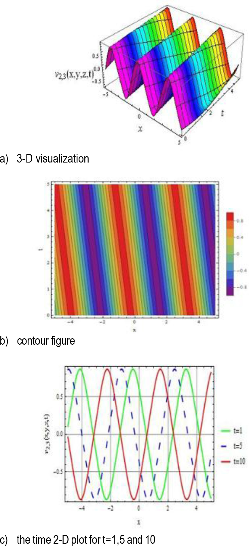
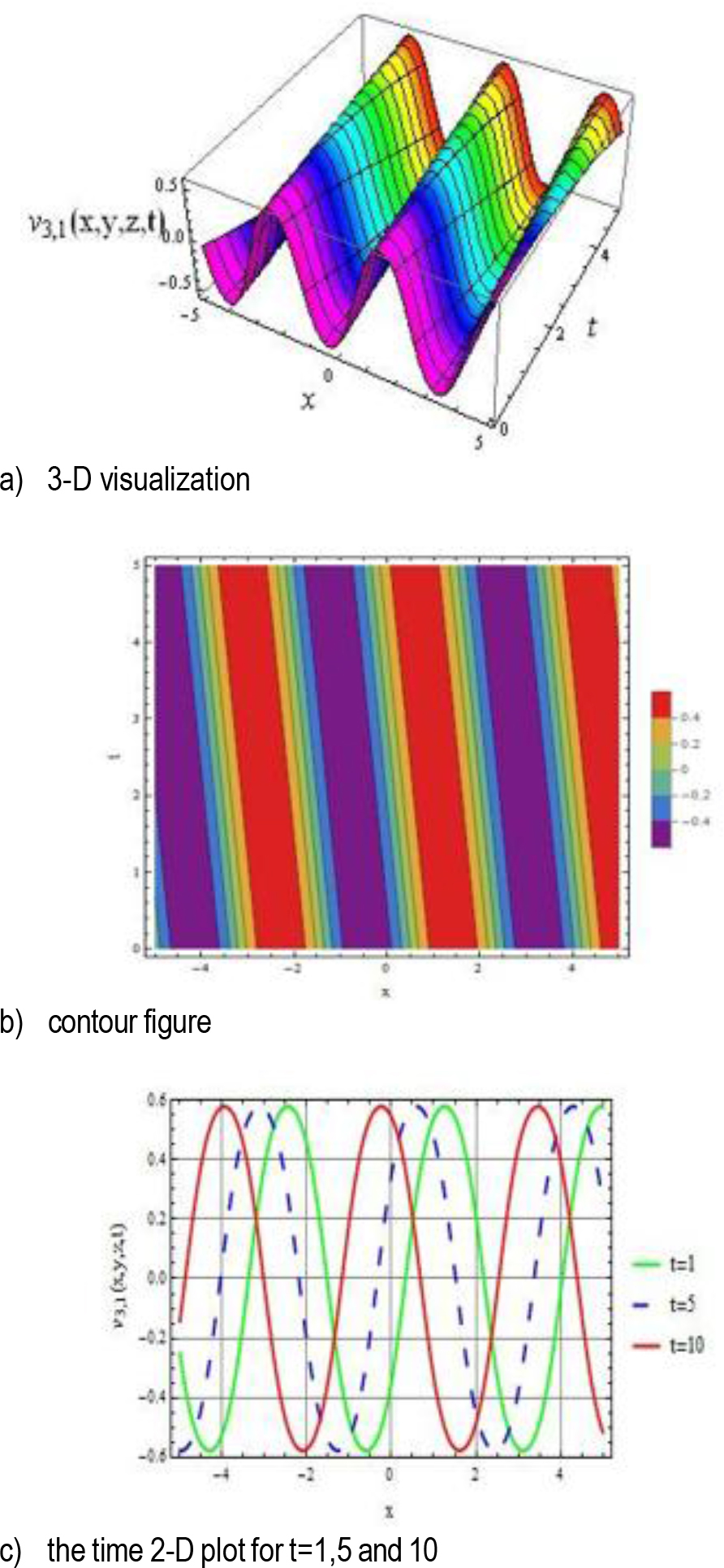
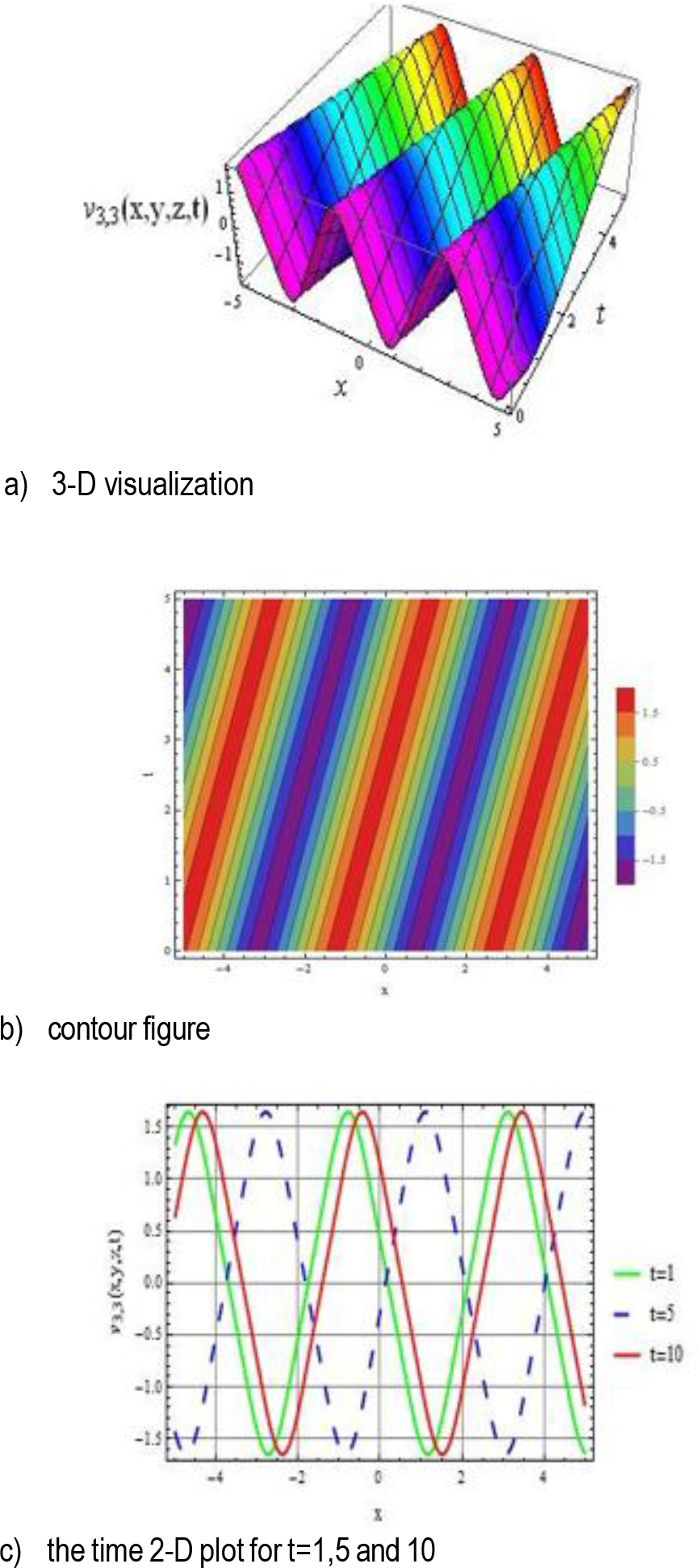
4. GRAPHICAL RESULTS AND DISCUSSION

In this section, we present several solution figures in 2-D, 3-D, and contour plots. All of the figures were created using Mathematica. The generalized JEFE technique yields novel solutions to the nonlin ear three-dimensional Wazwaz-Benjamin-Bona-Mahony (3D WBBM) equations, and its periodicity is proved. We illustrated many sorts of soliton structures, including steep kink, kink, peakon, rogue, and periodic soliton. The 2D plots show simplified cross-sections of the wave solutions, focusing on specific directions to highlight their oscillatory and (quasi-)periodic patterns. These views make it easier to observe changes in amplitude, phase, and frequency over time, helping us understand how the waves behave and evolve.

Fig. 1.

The 3-D visualization, contour plot, and 2-D graphical representation of V_1,1(x, y, z) are presented for the parameter values k = 0.5, r = 1, p = 2, q = –2, and y = z = 1

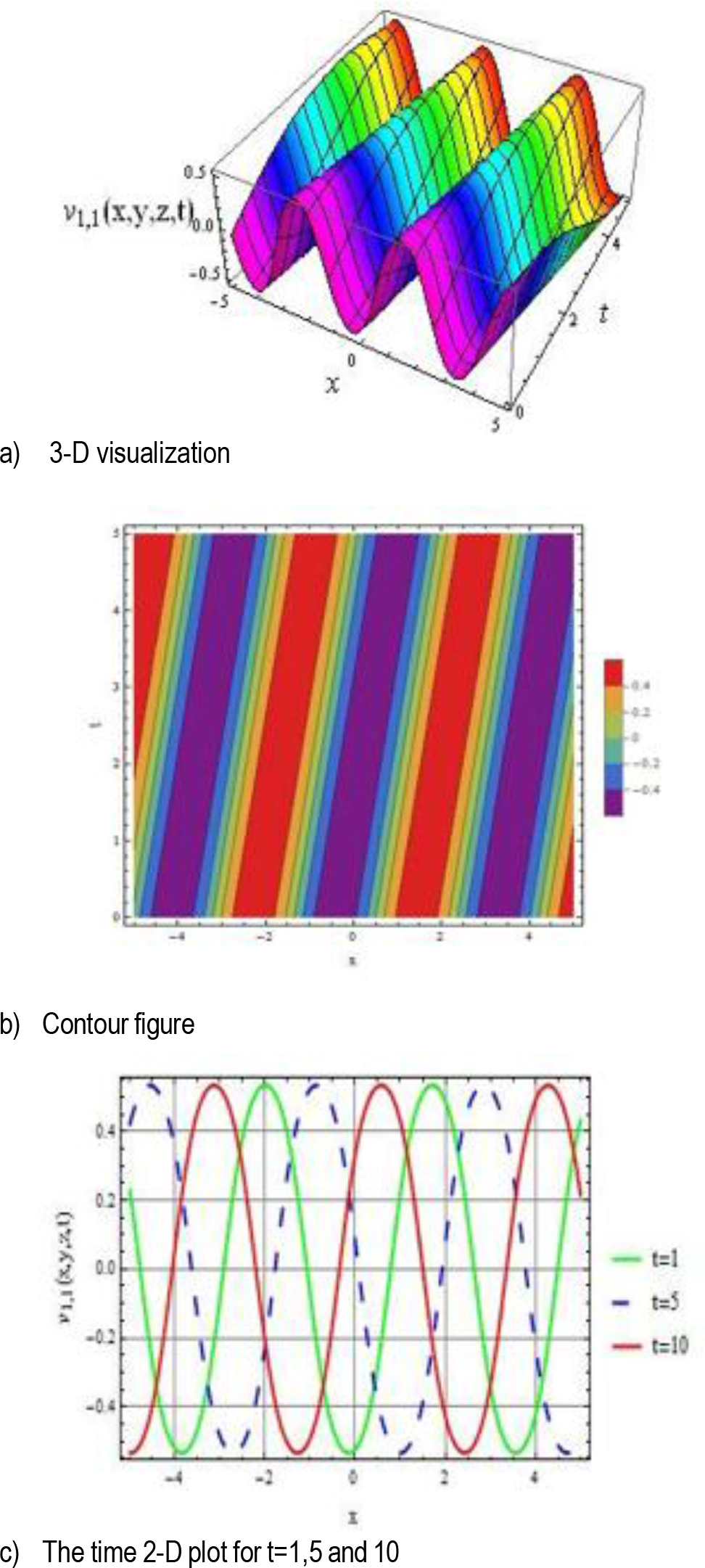
https://www.amajournal.com/f/fulltexts/213272/j_ama-2025-0048_fig_001_min.jpg

Fig. 2.

The 3-D visualization, contour plot, and 2-D graphical representation of v1,3(x, y, z) are presented for the parameter values k = 0.5, r = 0.5, p = 2, q = 2, and y = z = 1

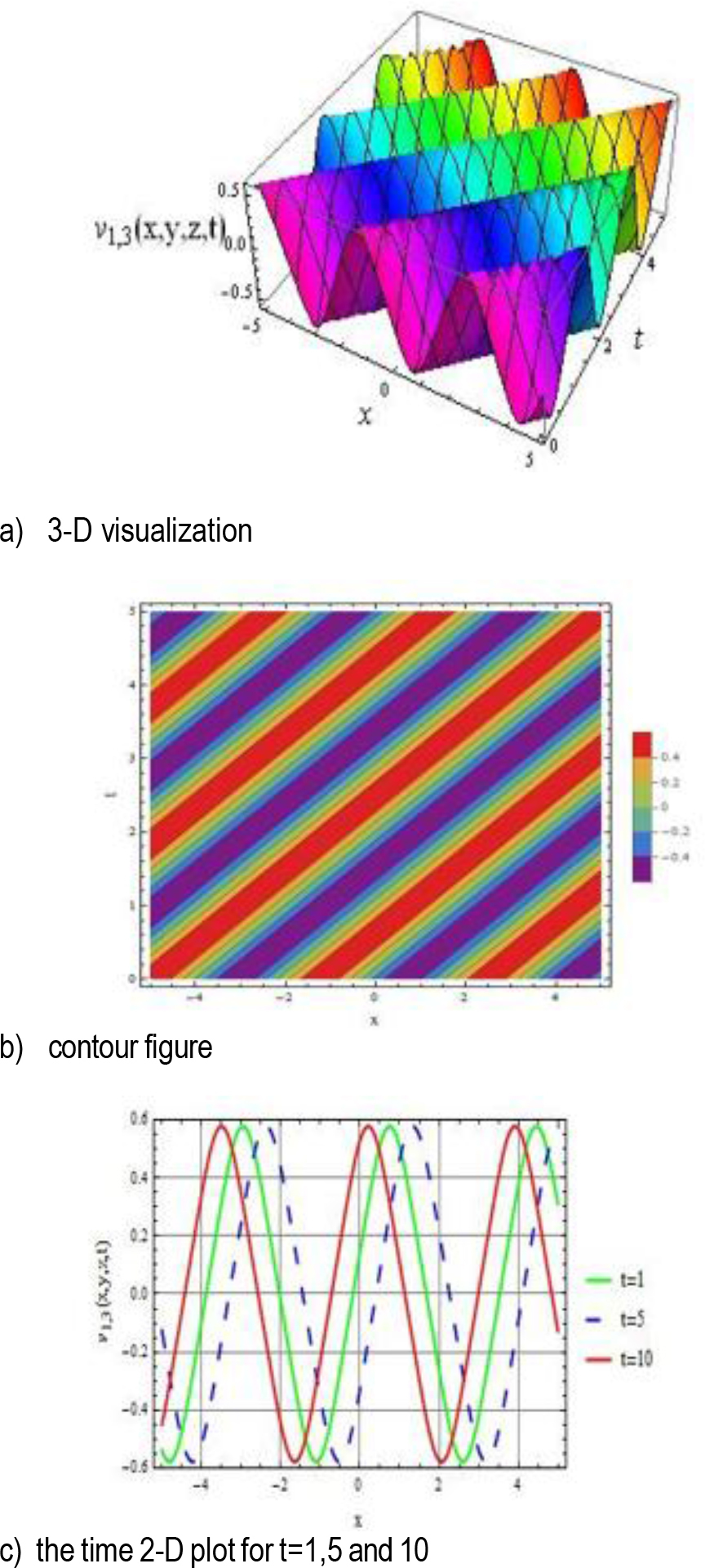
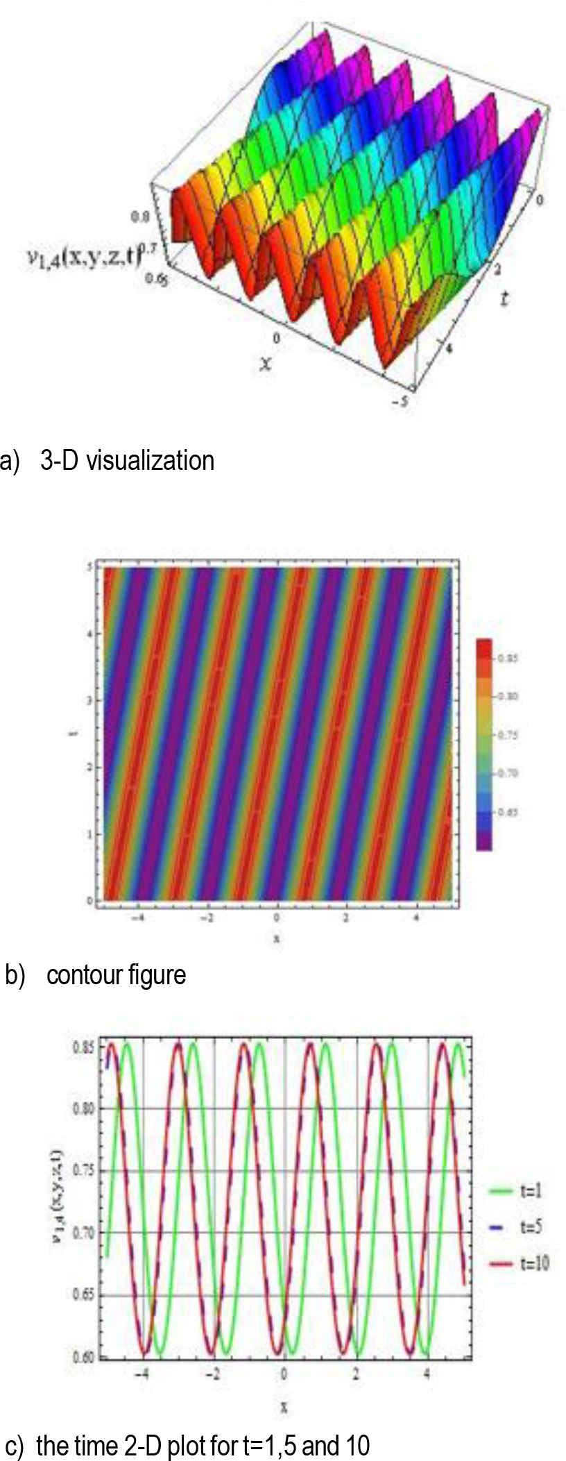
https://www.amajournal.com/f/fulltexts/213272/j_ama-2025-0048_fig_002_min.jpg

Fig. 3.

The 3-D visualization, contour plot, and 2-D graphical representation of V_1,4(x, y, z) are presen-ted for the parameter valuesk = 0.5, r = 0.5, p = 2, q = –2, and y = z = 1

https://www.amajournal.com/f/fulltexts/213272/j_ama-2025-0048_fig_003_min.jpg

The 3D surface plots clearly display how the wave’s height, frequency, and shape vary with different parameters, offering insights that are hard to see just from equations. Contour plots, which map the wave levels onto a flat surface, reveal the internal structure of the solutions, showing areas with steady values or sharp transitions. Together, these 2D, 3D, and contour plots give a fuller picture of the wave behaviors described by the 3D WBBM equations. Sub-sequently, the generalized JEFE process leads to more consistent results when addressing the WBBM equation, making it an effective tool for generating exact periodic and solitary wave-type soliton solutions.

Additionally, the Φ⁶-expansion and modified extended direct algebraic methods [31], and Khater method [32] to compute trigonometric, hyperbolic, Jacobi elliptic, and rational functions. The expanded tanh approach [33] was also applied to the bright, dark, periodic, and single soliton solutions. To differentiate this from the previous efforts. All our founded solutions are depending on the Jacobi elliptic functions and their corresponding hyperbolic and trigonometric functions. Jacobi elliptic function is a more generalized form of the hyperbolic and trigonometric functions.

This work is important for our research because it shows how effective the generalized Jacobi elliptic function expansion method is in analyzing and resolving intricate nonlinear systems. The tech-nique advances our knowledge of the dynamics at play in nonlinear systems by producing precise and physically meaningful solutions as well as making complex wave phenomena like solitons easier to visualize. The Jacobi elliptic function expansion approach is a strong and flexible tool for studying nonlinear wave dynamics.

Fig. 4.

The 3-D visualization, contour plot, and 2-D graphical representation of V_1,5(x, y, z) are presen-ted for the parameter values k = 0.5, r = 1, p = 2, q = 2, and y = z = 1

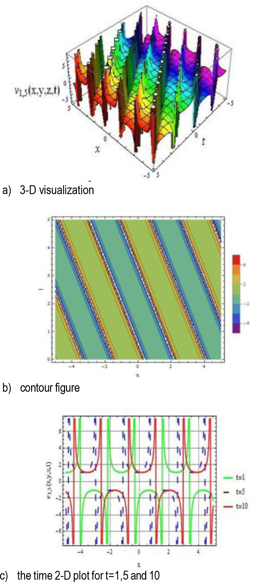
https://www.amajournal.com/f/fulltexts/213272/j_ama-2025-0048_fig_004_min.jpg

Fig. 5.

The 3-D visualization, contour plot, and 2-D graphical representation of V_1,11(x, y, z) are presen-ted for the parameter values k = 0.5, r = 1.5, p = –2, q = –2, and y = z = 1

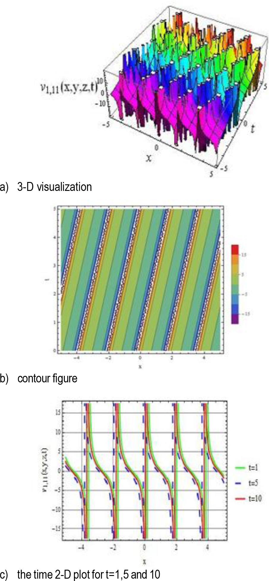
https://www.amajournal.com/f/fulltexts/213272/j_ama-2025-0048_fig_005_min.jpg

Fig. 6.

The 3-D visualization, contour plot, and 2-D graphical representation of V_1,26(x, y, z) are presented for the parameter values r = 2.5, p = 2, q = 𠀓2, and y = z = 1

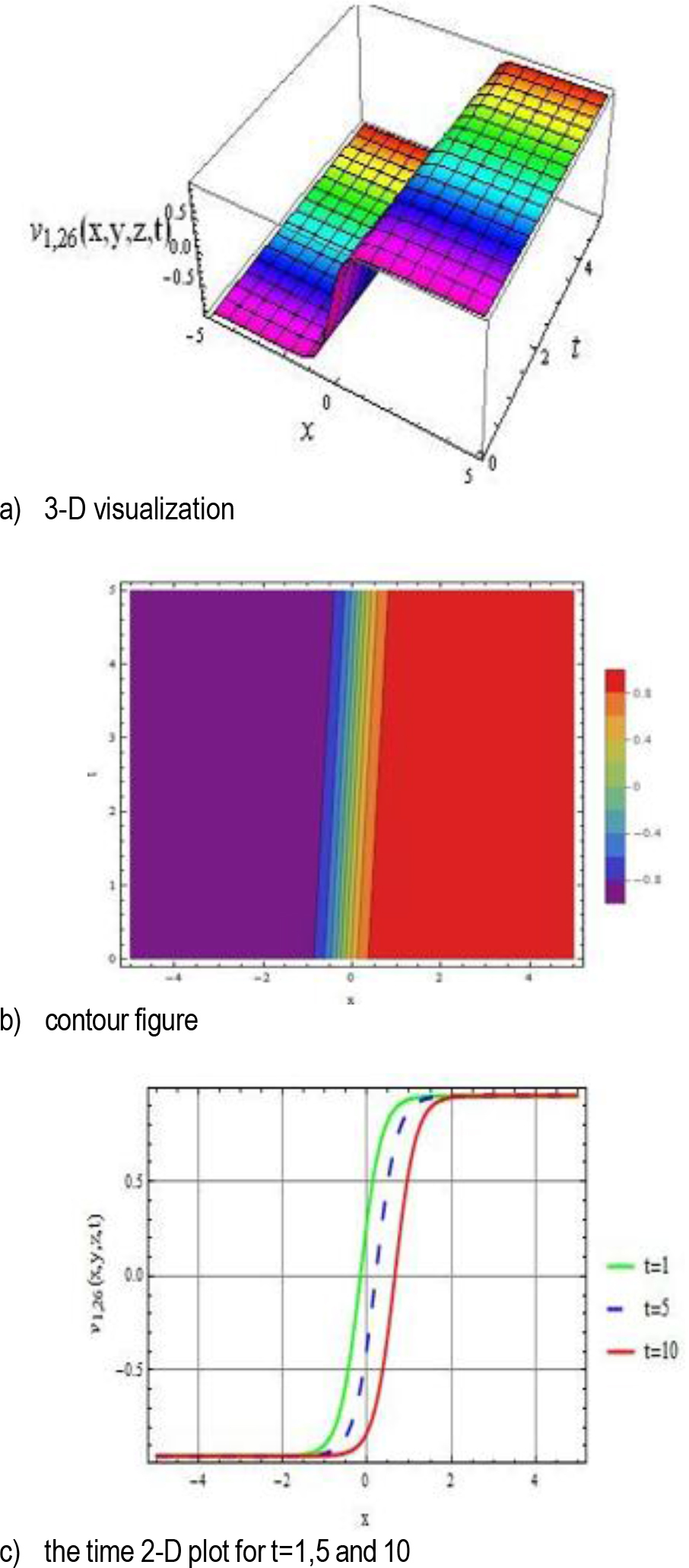
https://www.amajournal.com/f/fulltexts/213272/j_ama-2025-0048_fig_006_min.jpg

Fig. 7.

The 3-D visualization, contour plot, and 2-D graphical representation of V_1,27(x, y, z) are pre-sented for the parameter values r = 3, p = 1.5, q = –2, and y = z = 1

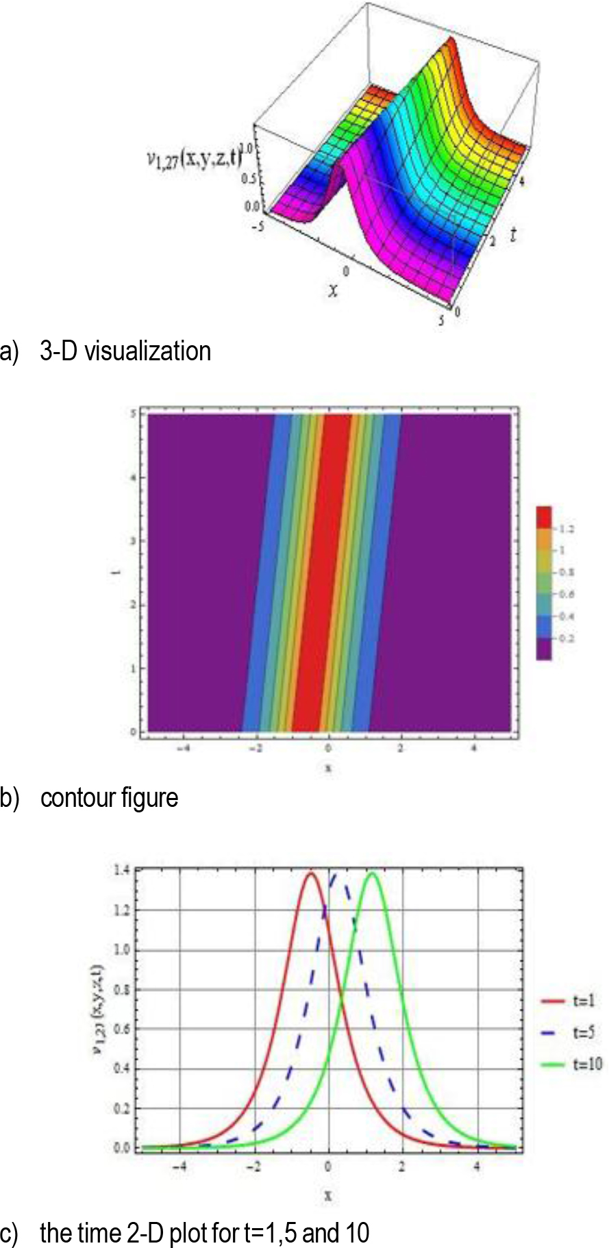
https://www.amajournal.com/f/fulltexts/213272/j_ama-2025-0048_fig_007_min.jpg

Fig. 8.

The 3-D visualization, contour plot, and 2-D graphical representation of V_1,29(x, y, z) are presen-ted for the parameter values r = 1.8, p = 1.5, q = –2, and y = z = 1

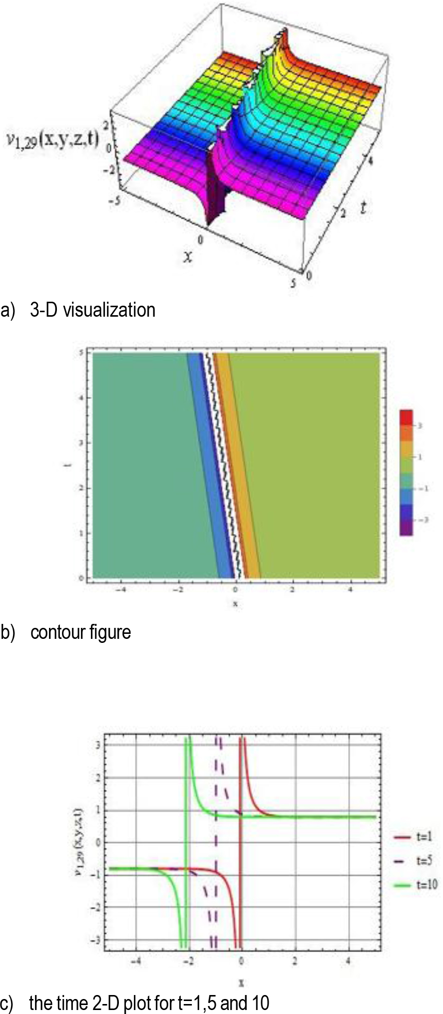
https://www.amajournal.com/f/fulltexts/213272/j_ama-2025-0048_fig_008_min.jpg

Fig. 9.

The 3-D visualization, contour plot, and 2-D graphical representation of V_1,40(x, y, z) are presented for the parameter values r = 1.8, p = 1.5, q = –2, and y = z = 1

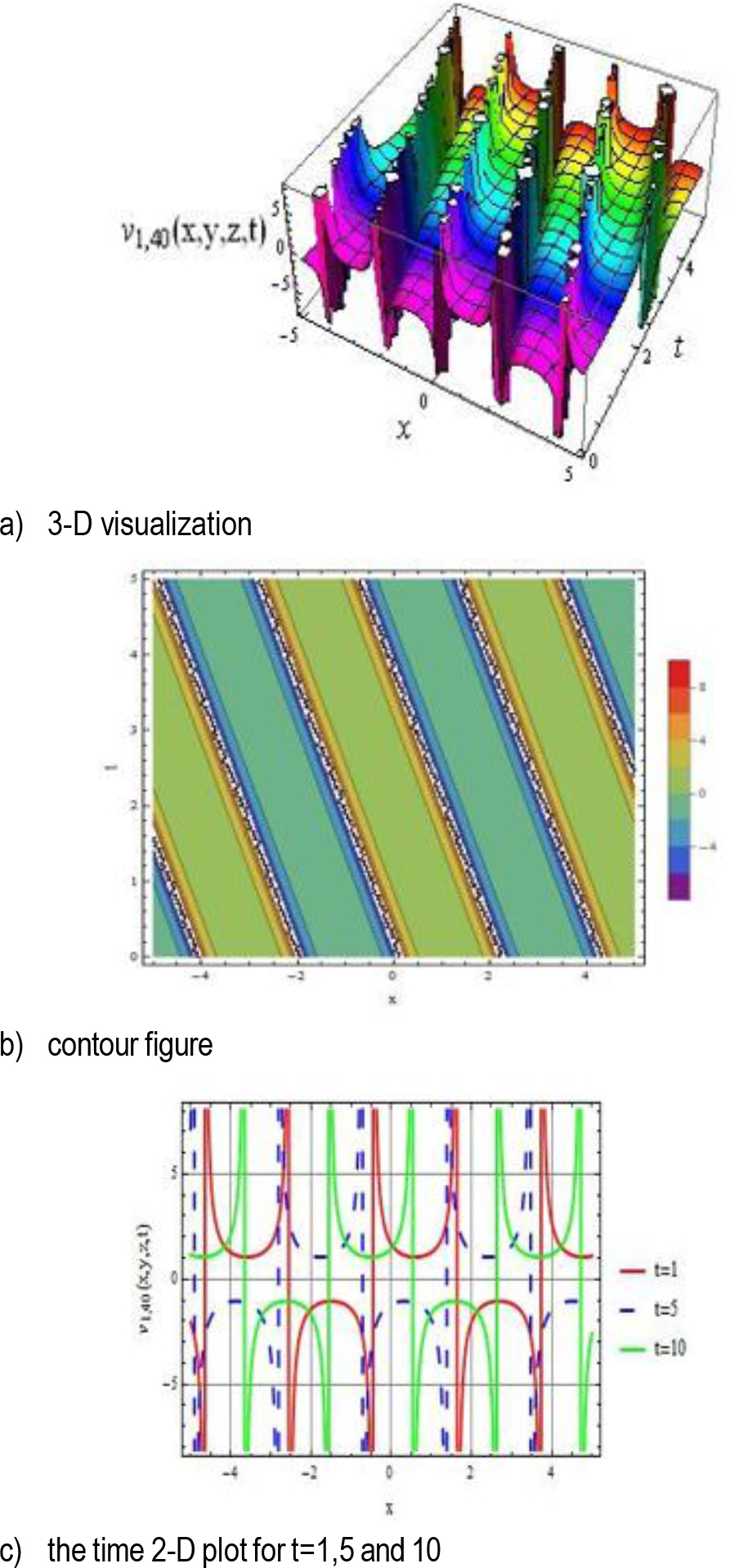
https://www.amajournal.com/f/fulltexts/213272/j_ama-2025-0048_fig_009_min.jpg

Fig. 10.

The 3-D visualization, contour plot, and 2-D graphical representation of V_1,41(x, y, z) are pre-sented for the parameter values r = 1.8, p = 1.5, q = –2, and y = z = 1

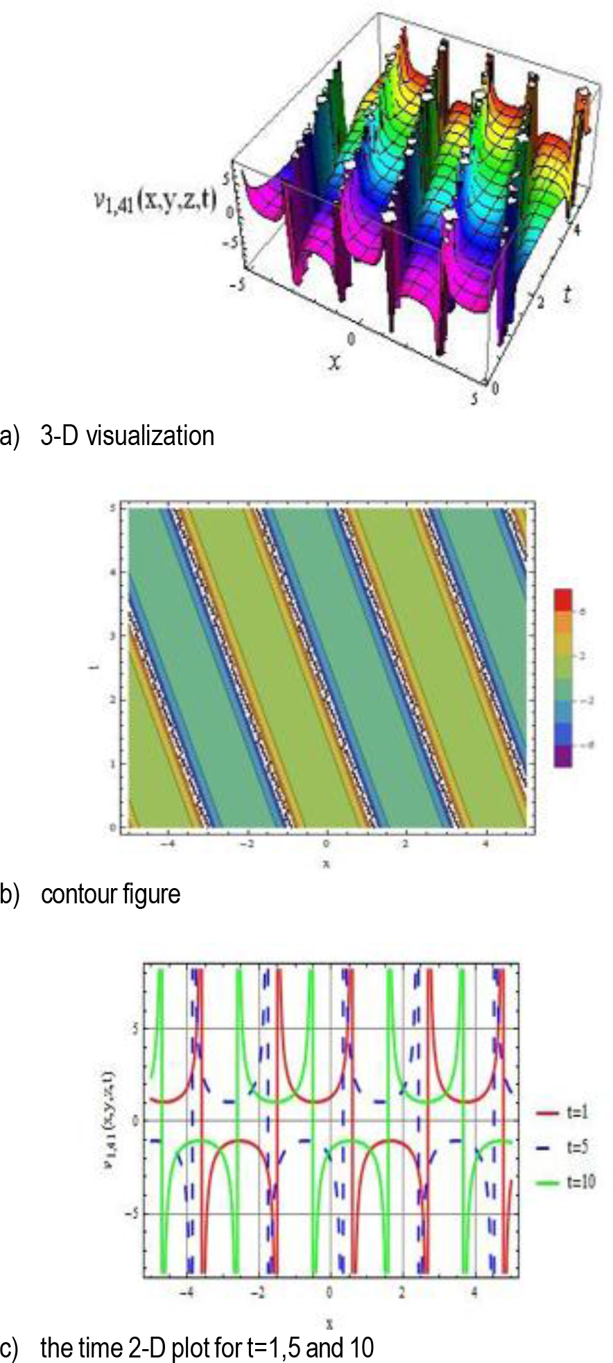
https://www.amajournal.com/f/fulltexts/213272/j_ama-2025-0048_fig_010_min.jpg

Fig. 11.

The 3-D visualization, contour plot, and 2-D graphical representation of V_1,43(x, y, z) are pre-sented for the parameter values r = 1.8, p = 1.5, q = 2, and y = z = 1

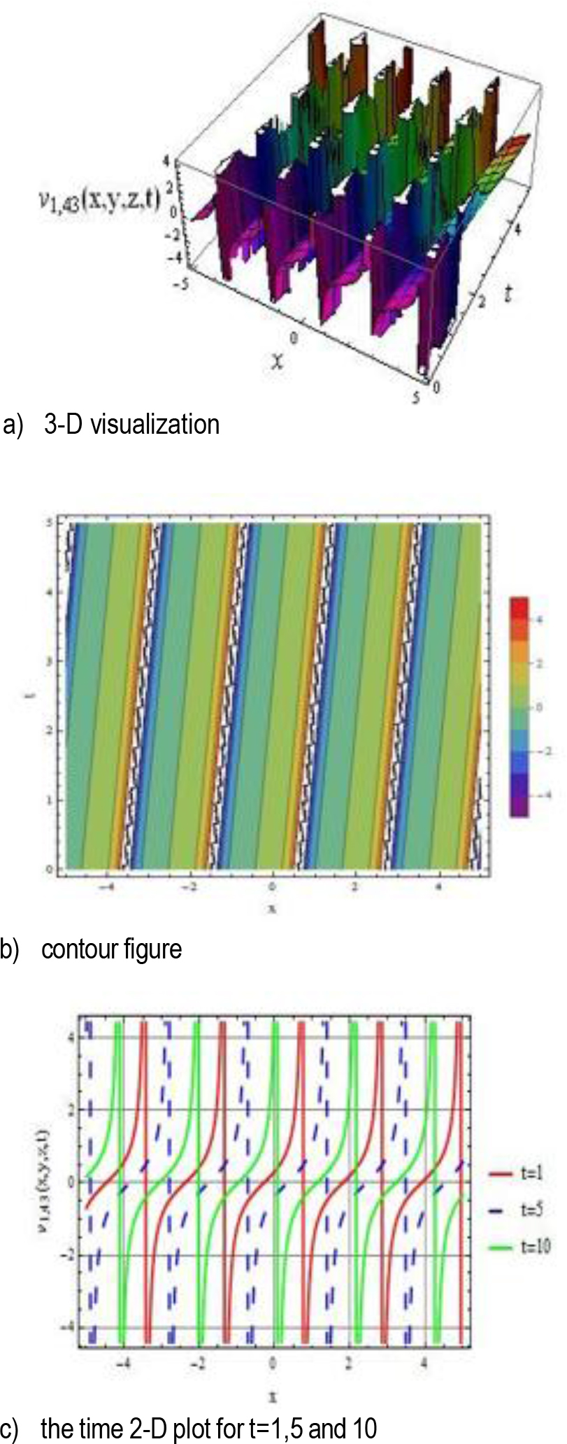
https://www.amajournal.com/f/fulltexts/213272/j_ama-2025-0048_fig_011_min.jpg

Fig. 12.

The 3-D visualization, contour plot, and 2-D gra-phical representation of V_2,1(x, y, z) are presented for the parameter values k = 0.5, r = –1, p = 2, q = 2, y = 1, and z = 1

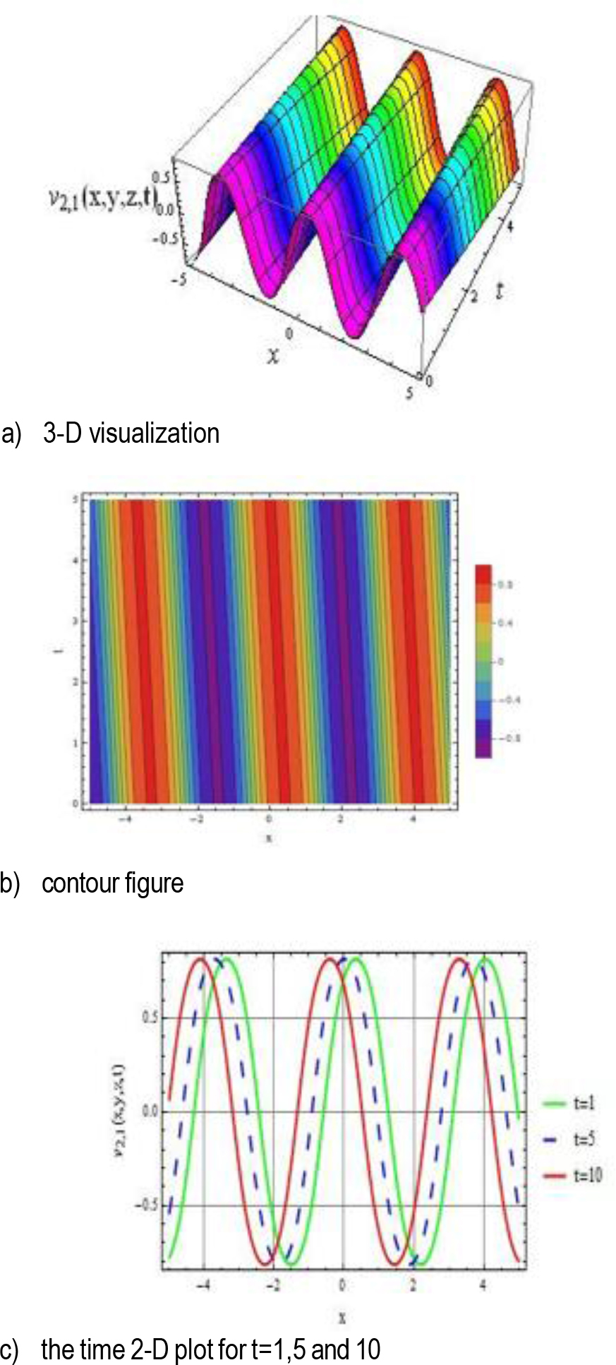
https://www.amajournal.com/f/fulltexts/213272/j_ama-2025-0048_fig_012_min.jpg

Fig. 13.

The 3-D visualization, contour plot, and 2-D graphical representation of V_2,3(x, y, z) are pre-sented for the parameter values k = 0.5, r = –1, p = 2, q = 1.5, y = 1, and z = 1

https://www.amajournal.com/f/fulltexts/213272/j_ama-2025-0048_fig_013_min.jpg

Fig. 14.

The 3-D visualization, contour plot, and 2-D graphical representation of V_3,1(x, y, z) are pre-sented for the parameter values k = 0.5, r = 1, p = 2, q = –2, y = 1, and z = 1

https://www.amajournal.com/f/fulltexts/213272/j_ama-2025-0048_fig_014_min.jpg

Fig. 15.

The 3-D visualization, contour plot and 2-D graphical representation of V_3,3(x, y, z) are presented for the parameter values k = 0.6, r = 0.5, p = 2, q = 2, and y = z = 1

https://www.amajournal.com/f/fulltexts/213272/j_ama-2025-0048_fig_015_min.jpg

5. CONCLUSION

The family of 3-D WBBM equations is efficiently solved in this work through the application of the generalized Jacobi elliptic function expansion technique. Through this method, the new periodic solutions are determined, which incorporates both solitary wave and shock wave solutions that have not been documented previously in the literature. These results give a greater understanding of the rich dynamic phenomena regulated by the family of 3-D WBBM equations, improving their applicability in fluid dynamics, nonlinear optics, plasma physics, and engineering. The obtained results have not been found in previous literature using this approach. To improve the physical description of the solutions several typical wave profiles are offered to provide a comprehensive analysis of the wave characteristics in 2-D, 3-D, and contour visualizations were generated using accurate parameters value with the help of Mathematica. Such graphical visualizations aid in our ability to more clearly understand and comprehend the system’s inherent features. The objective of this approach is quite applicative and powerful to analyze various soliton solutions, therefore it may be additionally applicable to many other nonlinear evaluation equations. Future research direction should focus to apply these approaches to additional complicated nonlinear systems to determine their broader application. Furthermore, investigating the stability and interactions of the generated solutions under different initial conditions and parameter changes might provide additional information. Furthermore, incorporating physics-informed neural networks represents a promising avenue for validating these solutions in practical applications, with the potential to bridge the gap between theoretical mathematics and real-world implementations in fields such as fluid dynamics, plasma physics, and engineering systems.

REFERENCES (42)

Qasim M, Yao F, Baber MZ, Younas U. Investigating the higher dimensional kadomtsev-petviashvili-sawada-kotera-ramani equation: Exploring the modulation instability, jacobi elliptic and soliton solutions. Physica Scripta. 2024.

Google Scholar

Hamza A, Suhail M, Alsulami A, Mustafa A, Aldwoah K, Saber H. Exploring soliton solutions and chaotic dynamics in the (3+1)-dimensional wazwaz-benjamin-bona-mahony equation: A generalized rational exponential function approach. Fractal and Fractional. 2024:592.

Google Scholar

Rahman Z, Ali MZ, Harun-Or-Roshid, Ullah MS. Analytical solutions of two space-time fractional nonlinear models using jacobi elliptic function expansion method. 2021.

Google Scholar

Alam MN, Hafez MG, Akbar MA, Harun-Or Roshid. Exact traveling wave solutions to the (3+1)-dimensional mkdv-zk and the (2+1)-dimensional burgers equations via exp(-ϕ(ξ)-expansion method. Elsevier BV. 2015.

Google Scholar

Hafez MG. Exact solutions to the (3+1)-dimensional coupled kleingordon-zakharov equation using exp(-ϕ(ξ)-expansion method. Elsevier BV. 2016.

Google Scholar

Akbar MA, Ali NHM, Zayed EME. A generalized and improved (G'/G)-expansion method for nonlinear evolution equations. Hindawi Publishing Corporation. 2012.

Google Scholar

Alzaidy JF. The (G'/G)-expansion method and travelling wave solutions for some nonlinear pdes. Am J Math Anal. 2013;1(3):28–32.

Google Scholar

Li X. Applications of F-expansion to periodic wave solutions for kdv equation.

Google Scholar

Li BA, Wang ML. Applications of f-expansion method to the coupled kdv system. 2005.

Google Scholar

10.

Almatrafi M. Solitary wave solutions to a fractional model using the improved modified extended tanh-function method. Fractal and Fractional. 2023:252.

Google Scholar

11.

Zahran EHM, Khater MMA. Modified extended tanh-function method and its applications to the bogoyavlenskii equation. Applied Mathematical Modelling. 2016;40(3):1769–1775.

Google Scholar

12.

Kumar S, Mohan B. A novel and efficient method for obtaining Hirota's bilinear form for the nonlinear evolution equation in (n+1) dimensions. Partial Differential Equations in Applied Mathematics. 2022;5:100274.

Google Scholar

13.

Ma WX. Soliton solutions by means of Hirota bilinear forms. Partial Differential Equations in Applied Mathematics. 2022;5:100220.

Google Scholar

14.

Mahak N, Akram G. Extension of rational sine-cosine and rational sinhcosh techniques to extract solutions for the perturbed nlse with kerr law nonlinearity. The European Physical Journal Plus. 2019;134.

Google Scholar

15.

Joseph S. Exact traveling wave doubly periodic solutions for generalized double sine-gordon equation. International Journal of Applied and Computational Mathematics. 2022;8.

Google Scholar

16.

Ray S. New analytical exact solutions of time fractional kdv-kzk equation by kudryashov methods. Chinese Physics B. 2016;25:040204.

Google Scholar

17.

Sadighi A, Ganji DD. Exact solutions of nonlinear diffusion equations by variational iteration method. Computers Mathematics with Applications. 2007;54:1112–1121.

Google Scholar

18.

Sahoo S, Ray S, Abdou M. New exact solutions for time-fractional kaup-kupershmidt equation using improved (G'/G)-expansion and extended (G'/G)-expansion methods. Alexandria Engineering Journal. 2020;59.

Google Scholar

19.

Naher H, Abdullah FA. New generalized and improved (G'/G)-expansion method for nonlinear evolution equations in mathematical physics. Journal of the Egyptian Mathematical Society. 2014;22(3):390–395.

Google Scholar

20.

Yang XF, Deng ZC, Wei Y. A riccati-bernoulli sub-ode method for nonlinear partial differential equations and its application. Advances in Difference Equations. 2015.

Google Scholar

21.

Kumar S, Kumar A, Wazwaz AM. New exact solitary wave solutions of the strain wave equation in microstructured solids via the generalized exponential rational function method. European Physical Journal Plus. 2020;135.

Google Scholar

22.

Wazwaz AM. Exact soliton and kink solutions for new (3+1)-dimensional nonlinear modified equations of wave propagation. Open Engineering. 2017;7(1):169–174.

Google Scholar

23.

Javeed S, Imran T, Ahmad H, Tchier F, Zhao YH. New soliton solutions of modified (3+1)-d wazwaz–benjamin–bona–mahony and (2+1)-d cubic klein–gordon equations using first integral method. Open Physics. 2023;21.

Google Scholar

24.

Zayed EME, Abdelaziz MAM. The modified exp-function method and its applications to the generalized k (n, n) and bbm equations with variable coefficients. Iranian Journal of Science. 2014;36:359–365.

Google Scholar

25.

Hamza AE, Suhail M, Alsulami A, Mustafa A, Aldwoah K, Saber H. Exploring soliton solutions and chaotic dynamics in the (3+1)-dimensional wazwaz–benjamin–bona–mahony equation: A generalized rational exponential function approach. Fractal and Fractional. 2024;8(10).

Google Scholar

26.

Mamun AA, Ananna SN, An T, Asaduzzaman M, Rana MS. Sine-Gordon expansion method to construct the solitary wave solutions of a family of 3D fractional WBBM equations. Results in Physics. 2022;40:105845.

Google Scholar

27.

Ullah N, Asjad MI, Hussanan A, Akgül A, Alharbi WR, Algarni H, Yahia IS. Novel waves structures for two nonlinear partial differential equations arising in the nonlinear optics via sardar-Sub-Equation method. Alexandria Engineering Journal. 2023;71:105–113.

Google Scholar

28.

Demirbilek U. On the solitary wave solutions of different versions of fractional 3d-wazwaz–benjamin–bona–mahony equations. İstanbul Ticaret Üniversitesi Fen Bilimleri Dergisi. 2023;22.

Google Scholar

29.

Akram, Seadawy RA, Rizvi STR, Younis M, Althobaiti S, Sayed S. Traveling wave solutions for the fractional Wazwaz–Benjamin–Bona–Mahony model in arising shallow water waves. Results in Physics. 2021;20.

Google Scholar

30.

Siddique I, Mehdi KB, Jarad F, Elbrolosy ME, Elmandouh AA. Novel precise solutions and bifurcation of traveling wave solutions for the nonlinear fractional (3 + 1)-dimensional wbbm equation. International Journal of Modern Physics B. 2023;37(02):2350011.

Google Scholar

31.

Bilal M, Ahmad J, et al. New exact solitary wave solutions for the 3d-fwbbm model in arising shallow water waves by two analytical methods. Results in Physics. 2021;25:104230.

Google Scholar

32.

Ali A, Ahmad J, Javed S. Solitary wave solutions for the originating waves that propagate of the fractional wazwaz–benjamin–bona–mahony system. Alexandria Engineering Journal. 2023;69:121–133.

Google Scholar

33.

Ahmad J, Rani S, Turki NB, Shah NA. Novel resonant multi-soliton solutions of time fractional coupled nonlinear schrödinger equation in optical fiber via an analytical method. Results in Physics. 2023;52:106761.

Google Scholar

34.

Qasim M, Yao F, Baber MZ, Younas U. Investigating the higher dimensional Kadomtsev-Petviashvili-Sawada-Kotera-Ramani equation: exploring the modulation instability, Jacobi elliptic and soliton solutions. Physica Scripta. 2025;100(2):025215.

Google Scholar

35.

Farooq A, Khan MI, Nisar KS, Shah NA. A detailed analysis of the improved modified Korteweg-de Vries equation via the Jacobi elliptic function expansion method and the application of truncated M-fractional derivatives. Results in Physics. 2024;59:107604.

Google Scholar

36.

Khan MI, Asghar S, Sabi'u J. Jacobi elliptic function expansion method for the improved modified kortwedge-de vries equation. Optical and Quantum Electronics. 2022;54(11):734.

Google Scholar

37.

Khan MI, Khan A, Farooq A. Analyzing the Kuralay-II equation: bifurcation, chaos, and sensitivity insights through conformable derivative and Jacobi elliptic function expansion. Physica Scripta. 2024;99(9):095210.

Google Scholar

38.

Khan MI, Faridi WA, Murad MAS, Iqbal M, Myrzakulov R, Umur-zakhova Z. The formation and propagation of soliton wave profiles for the Shynaray-IIA equation. acta mechanica et automatica. 2025;19(1).

Google Scholar

39.

El-Sabbagh M, Ali A. New generalized jacobi elliptic function expansion method. Communications in Nonlinear Science and Numerical Simulation. 2008;13:1758–1766.

Google Scholar

40.

Farooq A, Ma WX, Ishfaq M. Exploring exact solitary wave solutions of kuralay-ii equation based on the truncated m-fractional derivative using the jacobi elliptic function expansion method. Optical and Quantum Electronics. 2024;56.

Google Scholar

41.

Al-Muhiameed Z, Abdel-Salam E. Research article generalized jacobi elliptic function solution to a class of nonlinear schrodinger-type equations. Journal of Applied Mathematics. 2011;11.

Google Scholar

42.

Lai S, Lv X, Shuai M. The Jacobi elliptic function solutions to a generalized Benjamin-Bona-Mahony equation. Mathematical and computer Modelling. 2009;49(1-2):369–378.

Volumes and Issues

Indexes

Table of contents

1. INTRODUCTION 2. SUMMARY OF THE GENERALIZED JEFE APPROACH 3. MATHEMATICAL FORMULATION OF THE GENEERALIZED JEFE APPROACH 4. GRAPHICAL RESULTS AND DISCUSSION 5. CONCLUSION REFERENCES

eISSN:	2300-5319
ISSN:	1898-4088

1. INTRODUCTION

1.1

1.2

1.3

2. SUMMARY OF THE GENERALIZED JEFE APPROACH

2.1

2.2

2.3

2.4

Tab. 1.

2.5

2.6

2.7

3. MATHEMATICAL FORMULATION OF THE GENEERALIZED JEFE APPROACH

Analysis of the first WBBM equation

3.1

3.2

3.3

3.4

3.5

3.6

3.7

3.8

3.9

3.10

3.11

3.12

3.13

3.14

3.15

3.16

3.17

Analytical periodic solutions in terms of Jacobi elliptic functions (JEF)

3.18

3.19

3.20

3.21

3.22

3.23

3.24

3.25

3.26

3.27

3.28

3.29

3.30

3.31

3.32

3.33

3.34

3.35

3.36

3.37

3.38

3.39

3.40

3.41

3.42

Tab. 2.

Solitary wave solutions

3.43

3.44

3.45

3.46

3.47

3.48

3.49

3.50

3.51

3.52

3.53

3.54

3.55

3.56

3.57

Shock wave solutions

3.58

3.59

3.60

3.61