
INTRODUCTION
Nonlinearity is a fascinating phenomenon in nature, and scientists believe that nonlinear study is the most promising means of gaining a deeper understanding of how nature works. Investigating a wide range of nonlinear ordinary and partial differential equations is critical for mathematically describing complicated processes that change over time. These mathematical formulas are created in various fields, including economics, optical fibers, elasticity, plasma physics, solid-state physics, population ecology, infectious disease epidemiology, physics, and natural sciences. Soliton solutions of the previously mentioned phenomenon have been a fascinating and extraordinarily active topic of study for the past several decades, with the accompanying problem being the creation of exact solutions to a large variety of nonlinear partial differential equations. As a result, mathematics and physical scientists have made significant efforts to develop exact wave solutions to certain NLPDEs and various practical and potent strategies, including Hirota’s method [1][2][3][4], Backlund transformations [5], Pfaffian technique [6], the extended simplest equation approach [7], Riemann–Hilbert method [8][9], modified Sardar sub-equation method [10], physics-informed neural networks algorithm [11], a unified method [12], bilinear Bäcklund transformation [13], modified F-expansion method [14], the symbolic computation and Hirota method [15], and so on.
A soliton is a single, self-reinforcing wave that passes over a medium without ever dispersing or dissipating, preserving its shape and speed. Solitons are extremely stable and may maintain their form over long distances due to their unique nature. A lump solution is an analytical rational function solution that exists in all directions in space, and solitons are analytic solutions that are exponentially localized in all directions in space and time. They have previously been identified for nonlinear integrable equations.
A well-known partial differential equation used to model the disturbance of the surface of shallow water in the presence of solitary waves is the Korteweg-De Vries (KdV) equation. This equation incorporates leading-order nonlinearity and dispersion and can be used to study weakly nonlinear long waves. In shallow water, it describes small-amplitude waves with long wavelengths. The KdV equations have different types, such as the fifth-order KdV equation [16], the lattice potential KdV equation [17], generalized geophysical KdV equation [18], modified KdV equation [19], seventh-order KdV equation [20], Schwarzian KdV equation [21], and many others.
Recently, the generalized Korteweg-De Vries (gKdV) equation in two dimensions became known and read as follows:
whereLu and Chen [22] investigated this problem and found many distinct solutions in addition to integrability results. By modifying the preceding (2+1)-dimensional form (1), Ismaeel et al. [23], have created a new (3+1)-dimensional integrable gKdV equation.
where β, β1, γ are defined as non-zero constants. The Painlev’e test to reveal the integrability of the equation was used and found that when β = β1, the equation becomes integrable. Therefore, we haveThe multiple soliton solutions to the equation (4) were reported by authors in Ref. [23]. In this paper, we use Hirota’s method, which is a direct method to obtain multiple soliton solutions to integrable nonlinear evolution equations. It is also possible to determine multiple soliton solutions using other methods, such as inverse scattering transform [24] and various other techniques. The advantage of Hirota’s method over the others is that it is algebraic rather than analytic. Therefore, Hirota's method provides the most efficient results when we just want to construct multiple soliton solutions. Also, applying the long-wave method on N-soliton solutions, we can offer M-lump waves. In the present study, one-, two-, and three-M-lump waves, three interaction phenomena of soliton with M-lump waves, and four types of complex multiple solutions are derived. To our knowledge, these propagation wave solutions have not been investigated before.
Following is a summary of this study: In the second section, under the corresponding N-soliton solutions, the main idea is to construct M-lump solutions for equation (4), which is made possible by using a long wave method. In the third section, we offer and analyze the characteristics of mixed solutions, a mix of lump and soliton solutions. The fourth section is about the complex N-soliton solutions for the studied equation. In the fifth section, results and discussion about constructed solutions are presented. The last part contains some discussions and conclusions from this effort.
MULTIPLE M-LUMP SOLUTIONS
To extract the soliton solutions to the Eq. (4), consider the relation
Therefore, equation (4) could be shown to possess its bilinear form
where f = f(x, y, z, t) and D is the Hirota derivative and stated asThe notation ∑μ=0,1 represents the sum of all possible composites μm = 0,1, for = 1,2,…, N.
By taking the specific condition m < n, the first three solutions of Eq. (7) have the form
where with dispersion relation and whereHere km, lm, jm, wm, λm, are constants, whereas Ωm defines as the functions dependent on x, y, z, t. Now, to address the M-lump wave solution, we apply the long-wave method by taking N = 2, and assuming, km → 0, eλm = –1, and
Taking l1 = a1 + b1i,
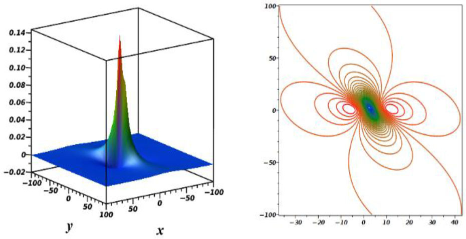
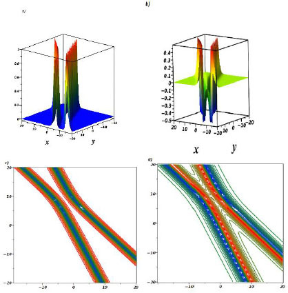
Equation (16) is a single M-lump wave as shown in Figure (1) for the gKdV equation with decaying as
Fig. 1.
Graphs of one-M-lump wave when z = 2, t = 2,
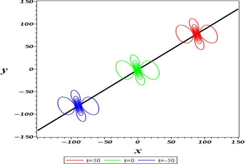
The path followed by this wave is denoted by the following plane:
whereThe one-M-lump wave on this plane is depicted in Figure (2) at various time periods.
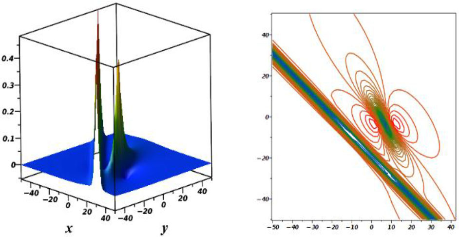
As part of our analysis of the equation, we want to specify the characteristics of a double-M-lump wave by considering N = 4 in Eq. (7), and km → 0, eλm = –1 (m = 1,2,3,4), the outcome offers
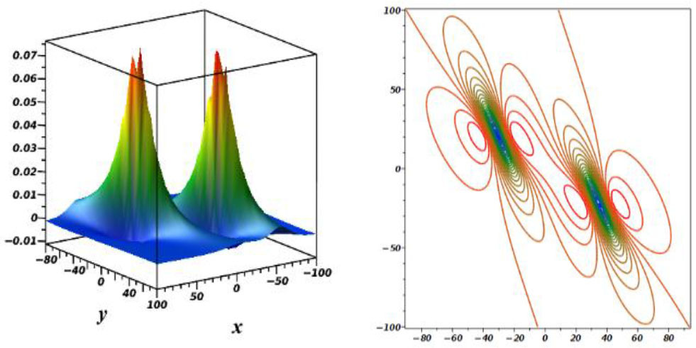
where Φ1, Φ2, Φ3, Φ4, wm and Bmn(n < m) are explained with Eqs. (13), (14), and Eq. (15), respectively. The double-lump solution is obtained by combining equation (17) with the other findings in equation (5) and demonstrated in Figure 3.Fig. 3.
Plots of 2-M-lump wave when z = 2, t = 2, a1 = 0.5, b1 = 0.5,
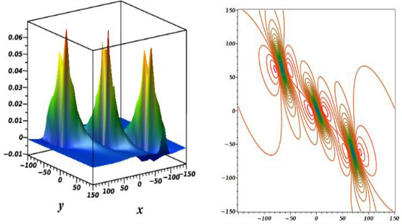
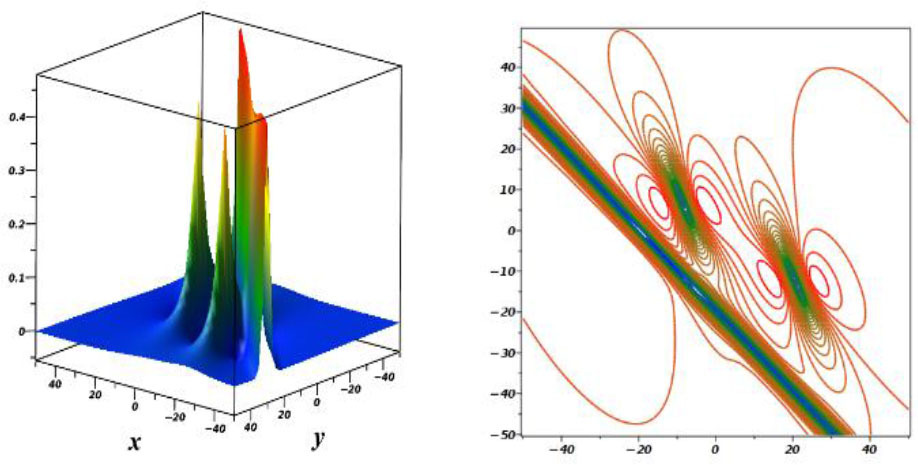
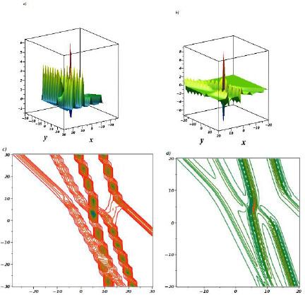
For 3-M-lump of Eq. (4), we take km → 0, eλm = –1 (m = 1,…,6) and considering N = 6 in Eq. (7), shows
18
We should know that Φp(p = 1,…,6), wm, and Bmn are depicted in Eq. (13), Eq. (14) and Eq. (15), respectively. By introducing Eq. (18) into Eq. (5), a 3-M-lump solution is displayed in Fig. 4. It is important to understand that l1 = a1 + b1i, l2 = l2 + b2i, l3 = a3 + b3i,
COLLISION PHENOMENA
Through a long-wave approach and setting km → 0, with
By combining Eq. (19) with Eq. (5), the outcome is a combination of a single-lump with a single-soliton solution (see Fig. 5).
Fig. 5.
Plots of M-lump with soliton solution when z = 1, t = 2, a1 = 0.5, b1 = 0.5,
Setting N = 4 in Eq. (7), and km → 0,
Eq. (22) can be substituted into Eq. (5) to provide a result that combines the properties of a double-soliton solution and a single-M-lump solution (refer to Fig. 6).
Fig. 6.
Graphs of M-lump with a 2-soliton solution when z = 1, t = 2, a1 = 0.5, b1 = 0.5,
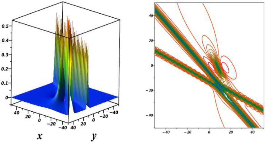
If N = 5 and taking the limit km → 0 and eλm = –1 for m = 1,2,3,4, in Eq. (7), we get
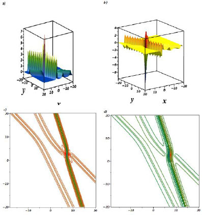
whereThe outcome shown in Figure 7 is the observable feature, which is obtained by combining Eq. (24) and Eq. (5) to illustrate an interaction of a two-M-lump with a soliton solution. A complete list of all constants and functions can be found in this article.
COMPLEX MULTI-SOLITON SOLUTIONS
Here, we explore the complexity of multi-solutions to the studied equation to explore new features of solutions.
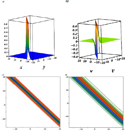
. The complex one-soliton wave
First, to construct the complex one-soliton wave, the assumption is
Substituting this assumption into Eq.(5), the result is
This solution is shown graphically in Fig. (8).
. The complex two-soliton solution
Here, the objective is to drive a double-soliton solution, where the assumption is
Putting this equation into Eq. (5), the result yields
where andThis solution represents a complex two-soliton solution, and it is drawn in Fig. (9).
. The complex three-soliton solution
To report a three-soliton solution in complex form, let
Substituting this equation into Eq. (5), we have
The function θm is defined as
with dispersion relation where the constant S123 =S12S13S23 S123 = S12S13S23.The constant Smn is stated as
whereThe result of this solution is presented in Fig. (10), which is a complex-three-soliton solution.
. The complex four-soliton solution
To report a four-soliton solution in complex form, let
34
This equation represents a complex four-soliton solution (see Fig. (11)). The research paper contains all required constants and functions.
Fig. 11.
Graphs of complex four-soliton wave are plotted for z = 1, t = 2, k1 = 1, k2 = 1, k3 = 2, k4 = 2, l1 = 1, l2 = 0.5,
RESULTS AND DISCUSSION
The gKdV equation has been investigated, and some novel solutions have been presented. A logarithmic variable transform is considered to transform the studied equation to the Hirota bilinear form. Via Hirota bilinear and long-wave methods, novel physical features to the considered equation are derived. The one-M-lump wave is shown in Fig. 1, and the motion of this wave, which moves on a straight line, is presented in Fig. 2. In Fig. 3 and Fig. 4, the double-, and triple-M-lump solutions have been drawn with the corresponding contour plots. Hybrid solutions are also derived. In Fig. 5 shows, mixed single soliton with a single M-lump wave, in Fig. 6 shows, mixed double soliton with a single M-lump wave, and Fig. 7 shows, mixed single soliton with a double M-lump wave with corresponding contour plots. Moreover, the complexiton soliton solutions are also constructed. In Fig. 8, the real and imaginary parts of a complex one-soliton solution are sketched. In Fig. 9, the real and imaginary parts of a complex two-soliton solution are drawn. The triple-soliton solution in complex form is derived in Fig. 10, and in Fig. 11, the behaviours of the four-soliton solution are presented.
CONCLUSION
We have considered the gKdV equation as a mathematical model of waves on shallow water surfaces. As far as macroscale processes and phenomena are concerned, KdV remains the most complete and arguably most useful model. First, the (3+1)-dimensional gKdV equation via variable transform is converted to the Hirota bilinear form. The M-lump wave solutions, namely one-lump, two-lump, and three-lump solutions, have been explored by applying the long-wave technique on the N-soliton solutions, which were constructed via the Hirota method. The interaction solutions via utilizing both Hirota bilinear and long-wave methods have been derived. These physical phenomena are one-soliton-lump, two-soliton-lump, and two-lump-soliton solutions. By virtue of the Hirota method, the N-complex-soliton solutions in complex form are constructed. The propagation characteristics of all gained solutions are shown graphically in 3D and contour plots. All phenomena presented in this work are verified by plugging them back into the studied equation. All presented physical phenomena are novel and have not been presented in the previously published study. In future work, these methods could be applied to more integrable NPDE and complex PDE to explore new features of solutions.