
INTRODUCTION
Fractional calculus is an extension of classical integer-order calculus that involves derivatives and integrals of non-integer (fractional) orders. The mathematical foundations of fractional calculus are presented in various monographs, such as [12], [13], and [14]. The applications of fractional calculus across various fields of science and engineering have attracted considerable attention in recent years. It has been used in areas such as mechanics, electrical engineering, biology, chemistry, and signal processing [13, 16, 18]. The fractional-order modeling of real-world phenomena are often more accurate than classical integer-order models. The theory of fractional systems is an expanding field that explores properties of systems, including stability, controllability, observability, realisability, and more [1, 2, 4, 7, 11, 15, 17, 19]. Standard and positive fractional linear systems have been discussed in monographs [8] and [10], respectively. A dynamical system is termed positive when its state variables and outputs take nonnegative values for any nonnegative inputs. Numerous models exhibiting positive behaviour can be found across fields such as engineering, biology, medicine, and economics. A comprehensive overview of research in positive systems theory is provided in [3, 6].
In the modelling process, compartmental linear systems are frequently used. These systems consist of separate compartments that are interconnected, each representing a subsystem containing a specific material. The transfer of material between compartments is governed by linear equations [5]. The fractional continuous-time compartmental systems have been studied in [9].
In this paper, fractional discrete-time compartmental time-invariant linear systems are introduced and analysed. To the best of the authors’ knowledge, the problems of controllability, observability, and eigenvalue assignment have not yet been addressed for fractional discrete-time linear systems. This paper extends the fractional-order systems theory to this concern. A key advantage of discrete-time fractional-order numerical models is their ability to describe complex dynamical systems with non-local, memory-based interactions, providing more accurate and nuanced representations. These models are suitable for real-world processes where the future state depends not only on the current value but also on the entire history of the system.
The structure of the paper is as follows. Section 2 provides the fundamental definitions and theorems related to fractional and positive linear systems. In Section 3, the concept of fractional discretetime compartmental linear systems is introduced. Section 4 is devoted to the analysis of controllability and observability of the proposed systems, while Section 5 addresses the eigenvalue assignment problem. Finally, concluding remarks are presented in Section 6.
The notation used in this paper is as follows: 𝕽 - the set of real numbers, 𝕽n×m - the set of n × m real matrices, Z+ - the set of nonnegative integers,
STANDARD LINEAR DISCRETE-TIME SYSTEMS
Let us consider a linear discrete-time system represented by the following equations.
with the initial condition x0, where xi ∈ 𝕽n represents the state vector, ui ∈ 𝕽m the control input, and yi ∈ 𝕽p the system output, while A ∈ 𝕽n×m, B ∈ 𝕽n×m and C ∈ 𝕽p×nare the corresponding system matrices.Definition 2.1. [6, 8] The linear system (2.1) is called (internally) positive if
Theorem 2.1. [6, 8] The linear system (2.1) is positive if and only if:
Definition 2.2. The linear system (2.1) is called asymptotically stable if
Theorem 2.2. [6, 8] The linear system (2.1) is asymptotically stable if the matrix A is a Schur matrix.
Theorem 2.3. [6, 8] The positive linear system (2.1) is asymptotically stable if and only if:
1. all coefficients of the polynomial
are positive, i.e., ai > 0 for i = 0,1,…, n – 1.2. there exists strictly positive vector
Let us now examine a linear fractional discrete-time system given by the following equations:
where xi ∈ 𝕽n, ui ∈ 𝕽p and yi ∈ 𝕽p are the state, input and output vectors and A ∈ 𝕽n×n, B ∈ 𝕽n×m, C ∈ 𝕽p×n and is the fractional α-order difference of xi.Substitution of (2.5b) into (2.5a) yields
whereDefinition 2.3. [6, 8] The fractional system (2.5) is called (internally) positive if
Theorem 2.4. [6, 8] The fractional system (2.5) is positive if and only if
Definition 2.4. [6, 8] The fractional positive system (2.5) is called asymptotically stable if
Theorem 2.5. [6, 8] The fractional positive system (2.5) is asymptotically stable if and only if one of the equivalent conditions is satisfied:
STATE EQUATIONS OF THE FRACTIONAL DISCRETE-TIME LINEAR COMPARTMENTAL SYSTEMS
Let us consider the compartmental discrete-time time invariant system consisting of compartments (Fig.1).
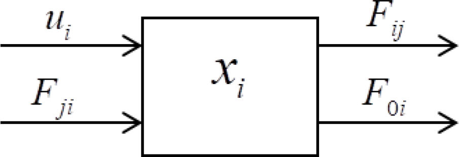
Let: xi = xi(k), x = 1, …, n be the amount of a material of the i -th compartmental at the time instant k,
Fij(k) > 0 be the output flow of the material from the j -th to the i -th compartmental (i ≠ j), between the k -th and k + 1-th time instants,
F0i(k) > 0 be the output of the material from the i -th (i = 1,…, n) compartmental to the environment,
ui = ui(k) be the output flow of the material to the i -th compartmental from environment.
It is assumed that the input material is instantaneously mixed with the material already present in the compartment and that Fij(k) depends linearly on x(k), i.e.,
where fij is a coefficient depending on xj(k) and the discrete-time instant k.The system is linear if fij is independent of xj(k) and it is additionally time-invariant if fij is independent of k.
From the balance of material of the i -th compartment we have the following fractional difference equation
where Δαxi is defined by (2.5b) and xi(k) denotes the amount of material in the i -th compartment at time step k, i.e.,From equation (3.3) we have
Note that if uj(k) = 0, then the output flow of material from the -th compartment at the time instant k + 1 cannot exceed the total amount of material present in the compartment at time instant k, i.e.,
Definition 3.1. The matrix
Using (3.3) for i = 1, …, n we obtain the state equation of the compartmental system in the form
whereThe output equation of the compartmental system has the form
whereFrom (3.6) it follows that the fractional compartmental systems are positive linear systems.
CONTROLLABILITY AND OBSERVABILITY OF STANDARD AND COMPARMENTAL LINEAR SYSTEMS
Let us consider a linear discrete-time system described by the following equations:
with the initial condition x0, where xi ∈ 𝕽n, ui ∈ 𝕽m and yi ∈ 𝕽p are the state, input and output vectors and A ∈ 𝕽n×n, B ∈ 𝕽n×m and C ∈ 𝕽p×n are system matrices.Definition 4.1. The linear system (4.1) (or the pair (A, B)) is called controllable in the interval time [0, if] = 0,1, …, if if the exists an input ui for i ∈ [0, if] which steers the state of the system from initial state x0 ∈ 𝕽n to the given final state xf, i.e., xif = xf.
Theorem 4.1. The linear system (4.1) is controllable if and only if one of the following conditions is satisfied:
where C is the field of complex numbers.Definition 4.2. The linear system (4.1), or equivalently the pair (A, C), is called observable if it is possible to uniquely determine the initial state x0 based on the input ui and output yi for i = 0,1,…, if.
Theorem 4.2. The linear system (4.1) is observable if and only if at least one of the following conditions is satisfied:
Now let us consider the fractional compartmental linear system (3.6)
Definition 4.3. The fractional compartmental linear system (3.6), or equivalently the pair (F, B), is called reachable on the time interval [0, if] if there exists an input sequence ui for i ∈ [0, if] which steers the system state from the zero initial condition to a given final state xf, i.e., xif = xf.
A matrix F ∈𝕽n×n is called monomial if each of its rows and each of its columns contains exactly one positive entry, and all other entries are zero.
Theorem 4.4. The fractional compartmental linear system (3.6) is reachable if the matrix
is monomial. The input which steers the system state to xif = xf is given byProof. When matrix (4.6) is monomial, its inverse
since B = In.
Therefore, the input (4.7) steers the state of the system from x0 to xif = xf.
Theorem 4.5. The fractional compartmental positive linear system (3.6) is reachable in time [0, if] if and only if the matrix F ∈ Mn is monomial.
Proof. Sufficiency. If F ∈ Mn is monomial then
Necessity. From Cayley-Hamilton theorem [6] we have
where aij are some nonzero real coefficients.Using (4.10) we obtain
whereTherefore, for given
Observe that for the nonnegative system defined in (4.11b), a nonnegative input
Observability of fractional positive compartmental linear systems is defined analogously to that in standard positive linear systems. Since it is determined exclusively by the matrices A and C, and not by B. Consequently, system (2.1) is replaced by the fractional positive compartmental linear system of the following form
where xi ∈ 𝕽n, yi ∈ 𝕽p andThe solution to the equation (4.13a) with (2.6b) has the form
where with Φ0 = In.Definition 4.4. The fractional positive compartmental linear system (4.13) is called observable on the interval [0, if] if knowledge of the output yi over the interval [0, if] enables unique determination of the initial state x0.
Theorem 4.6. The fractional positive compartmental linear system (4.13) is observable on the interval [0, if] if and only if the matrix
is monomial.Proof. Substituting (4.14a) into (4.13b) we obtain
Note that
EIGENVALUE ASSIGNMENT IN THE STANDARD AND FRACTIONAL COMPARMENTAL LINEAR SYSTEMS
Let us consider the fractional compartmental system (3.3) under state feedback control
where K ∈ 𝕽n×n.Assuming B = In, it follows from equation (5.1) that
whereBased on the given matrix A and the desired close-loop matrix Ac from (5.3), the following expression can be derived
Accordingly, the following theorem is established.
Theorem 5.1. Given the fractional compartmental system (3.3), there always exists a state feedback (5.1) such that the closed-loop system matrix Fc achieves a specified set of eigenvalues.
Example 5.1. The matrix of the fractional compartmental linear system is given by
and its eigenvalues are: z1 = z2 = 2, z3 = –1, sinceDetermine the feedback matrix K ∈ 𝕽3×3 such that the closed-loop system matrix Fc has eigenvalues:
It should be noted that the desired closed-loop matrix Fc is not unique. Two alternative forms of Fc are considered below.
Case 1. The matrix Fc is assumed to be in the Frobenius canonical form, as in equation (5.5)
In this case using (5.4), (5.5) and (5.6) we obtain
Case 2. The matrix Fc Fc is assumed to be diagonal
In this case we have
Note that the presented approach can be generalized to include output feedback strategies.
CONCLUDING REMARKS
Fractional, compartmental, time-invariant linear systems are analyzed, with a focus on their fundamentalproperties. Theoretical foundations, including key definitions and theorems related to standard and positive fractional linear systems, are outlined. A class of fractional compartmental discrete-time systems is introduced and studied. The concepts of controllability and observability are discussed for both standard and compartmental systems, followed by an examination of the eigenvalue assignment problem in the compartmentalcase. The results obtained may also be extended to descriptor discrete-time fractional linear systems.