
INTRODUCTION
In recent years, fractional calculus has gained considerable attention among researchers in various fields of science and technology. This calculus deals with the general extension of the concept of differentiation and integration to non-integral orders, which makes it possible to analyze and model complex phenomena that are not fully described by classical equations [1, 2, 3, 4, 5]. However, the greatest potential of fractional calculus lies in its application to systems modeling and control, where the possibility of designing much more robust and accurate control systems emerges. Current research indicates that fractional-order controllers can achieve much better values of control quality indicators and are more resistant to changes in model parameters than the commonly used classical PID controller [2, 6, 7, 8, 9, 10, 11, 12, 13], but most industrial solutions available on the market use PI/PID-type controllers without achieving optimal performance. This fact is due to the difficulty of understanding the complexity of non-integer order controllers by the personnel operating the system and the complexity of implementing control algorithms in classical microcontrollers or other commercial devices. With the coming of Industry 4.0 [14] the automation industry is looking for new solutions to increase overall efficiency; that is why this paper will present both the recent available tools and implementation options for non-integer controllers.
The purpose of this article is to compile key theoretical foundations of fractional-order calculus, provide an overview of current trends in its practical applications, and demonstrate an example implementation of Fractional-order PID controller on myRIO-1900 measurement board.
In this paper, all necessary theoretical aspects related to fractional-order calculus and its application in automatic control systems will be presented. The most popular types of fractional-order controllers, methods for approximating fractional order, and current tuning methods for such controllers will be discussed. This will be followed by an analysis of current trends in hardware implementation of fractional-order controllers, along with an indication and comparison of available hardware and software tools. These tools were used to obtain models, the responses of which were compared with the response of a model of an object with fractional-order dynamics, called fractance, in order to determine the best one. The best tool will be used to develop an automatic control system with both a classical PID controller and a fractional-order controller, both in simulation and in the laboratory, and their results will eventually be compared. Both types of controllers will be tuned using the Modified Grey Wolf optimization algorithm.
FRACTIONAL CALCULUS
The fractional calculus is a form of generalization of the operations of integration and differentiation, through a new operator
There are many definitions of fractional operator, but they are used in different fields, making it easier to analyze the relevant functions. Currently, the most popular definitions found in modern books describing fractional calculus are the Riemann-Liovile definition RL, the Grünwald-Letnikov definition GL and the Caputo definition C.
Definition 2.1. A function given by the integral [1]
is called the Euler gamma function and satisfies the equality where R(x) is real part of complex number x.Definition 2.2. Riemann-Liouville fractional-order derivative is defined as [1]
Definition 2.3. Grünwald–Letnikov fractional-order derivative is defined as [4]
Definition 2.4. Caputo fractional-order derivative is defined as [1]
Due to its form, the Riemann-Liouville definition is used for relatively simple functions (xa, ex, sin(x), etc.), while Grünwald-Let-nikov definition found its use in numerical evaluation. On the other hand, because of its ability to consider time delays, memory effects, and the possibility of using the same form of initial conditions as for the integer-order case, the Caputo definition has found wide application in control theory and automation. In this paper, the Caputo definition will be used precisely because of the aforementioned properties.
Definition 2.5. The formula for the Laplace transform of the q–th order Caputo derivative eq. (2.6), when (N – 1 ⩽ q < N) has the form [1]:
Given that the function f(t) and all its derivatives have zero initial conditions f(0) = 0 when t = 0, then transform of the q–th order Caputo derivative can be simplified to sqF(s).
FRACTIONAL-ORDER CONTROLLERS
Controllers are an integral part of systems that provide process control using feedback loops. Fractional-order controllers, which are a generalization of classical integer-order controllers, are becoming increasingly popular. The leading types of Fractional-order controllers [4] today are CRONE Controller developed by Oustaloup in 1995, Fractional-order PID controller proposed by Igor Podlubny, and a number of lesser used controllers; Fractional lead-lag compensator (Raynaud and Zegaïnoh, 2000), non-integer integral (Manabe, 1961) and TID compensator (Lurie, 1994). In this paper only FOPID controller will be considered due to its relative simplicity.
. FOPID Controller
Fractional-order PIλDμ controller (FOPID) [3, 4] was first introduced in 1999 by Igor Podlubny as generalization of the classical PID controller with integrator of real order λ and differentiator of real order μ.
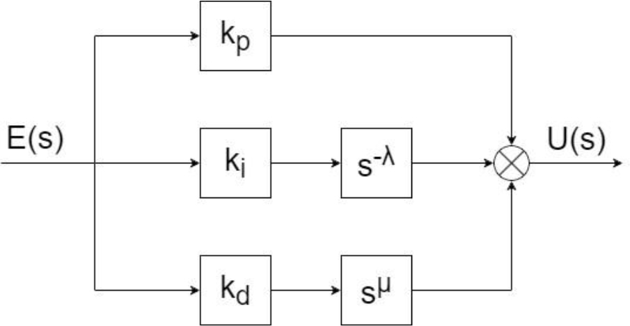
Definition 3.1. The FOPID Controller [4, 15] transfer function can be defined in time domain as:
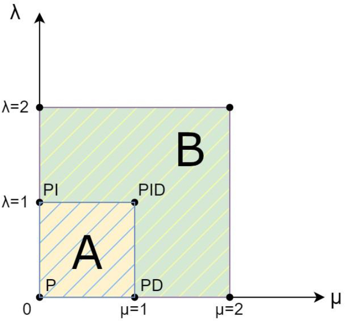
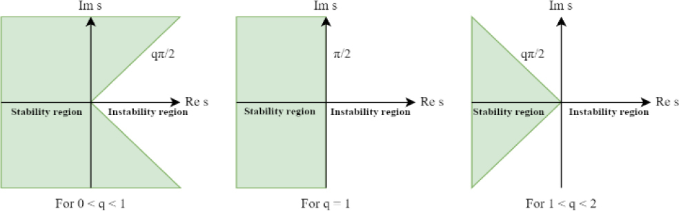
where, kp, ki, kd are proportional constant, integration constant and differentiation constant respectively.The general structure of FOPID Controller corresponding to eq. (3.1) is shown on Figure 3.1, where E(s) is control error and U(s) is controller output. In special circumstances PIλDμ controller can be equal to the classic PID Controller, for example if λ = 1 and μ = 0, then eq. (3.1) will describe PI controller as shown in Figure 3.2. The controller plane for FOPID has to be divided into two areas: A when 0 < λ, μ ⩽ 1 and B when 1 < λ, μ ⩽ 2. This is due to the stability conditions [16] of the system depending on the value of the controller order. In Figure 3.3, where q corresponds to fractional operator order, stability regions are depicted for the controller order corresponding to the zones separated in Figure 3.2. It is worth mentioning that using λ, μ > 2 will result in controllers instability.
. Approximation
For practical implementation of fractional integro-differentiator of order α it is necessary to use conventional transfer function approximation. One of such approximation methods is Oustaloup recursive filter [2,3], which provides very good results in specified frequency range (ωb; ωh) using the following equations:
where, N - order of approximation, ωh - higher bound of frequency fitness, ωb - bottom bound of frequency fitness.For digital implementation it is possible to use any suitable method for conversion to discrete-time equivalent.
. Controller tuning methods
The most challenging part of working with FOPID controllers arises when tuning them with the addition of two parameters related to the orders of integration and differentiation. The authors of the book [3] state that the known principles of the Ziegler-Nichols tuning method for the classical PID, can be applied to FOPID controllers for the values of constants kp, ki, kd, while the orders of λ and μ must be selected experimentally. However, this creates a difficulty in obtaining optimal system performance, as well as requiring the selection of the appropriate type of controller before the tuning process begins, as each controller (P, PIλ, PDμ, PIλD) provided significantly different results. They also proposed an analytical tuning method which is as follows:
Consider the mathematical model of a given plant
Since open-loop transfer function L(s) = C(s)G(s), the controller transfer function C(s), that gives the Bode’s ideal loop transfer function
takes the form: which can be expressed asThe transfer function eq. (3.9) is basically a IαDμ controller (where μ = 1–α). The time-domain equation of the controller C(s) is:
The open-loop transfer function L(s) = C(s)G(s) can then be described as
To obtain α and Kp the following procedure has to be used:
Find the fractional order α by using formula:
from the desired phase margin φm.Calculate the proportional gain Kp by using formula:
from the gain-crossover frequency ωcg and nominal gain of the system K. This method was verified by experiment conducted by the authors which proved that the system behaved according to designed specifications.
In [17] the extension of Z-N tuning rules was presented, in which the authors pointed out new more complex rules. They stated that by formulating five design criteria—target gain crossover frequency ωcg, desired phase margin φm, high-frequency noise attenuation, disturbance rejection, and robustness to plant gain variations—the parameters of a FOPID controller can be systematically computed.
The first criterion is posed as the objective function, while the remaining four are treated as constraints, resulting in a constrained optimization problem. This solution can provide good results in most cases but tends to reach local minima. However those results strongly depend on initial estimates of parameters provided, which is an important drawback, because in some cases finding the solution without well-chosen initial estimates can be difficult. The Authors tested those tuning rules on three different theoretical plants; first-order, second order and fractional-order. The experiment proved the usefulness of these rules and at the same time showed that, as in the case of the classical Z-N method, the resulting settings offer inferior performance to the one sought but can be applied even without knowledge of the plant model.
The last approach presented in [18] focuses on solely optimization algorithms. The authors considered BLDC (brushless direct-current) motor as a control plant and used PID and FOPID controller tuned with multiple different methods to test the performance of such system. They used genetic algorithm, fuzzy logic, Grey Wolf Algorithm, Artificial bee colony algorithm, Neural-networks and more, with all of them using the same conditions and cost functions. The most popular cost functions are defined with integral indexes, for example, Integral Absolute Error (IAE), Integral of Time Multiplied Squared Error (ITSE), Integral of Time Multiplied Absolute Error (ITAE). Each algorithm generated a certain controller set vector and then determined the value of the cost function, which it minimized at the next iteration. The main difference between the aforementioned solutions was the difference in the operation of the algorithm’s core, which handled the generation and updating of new set vectors. According to the results obtained by the authors, all of the considered methods can be successfully applied to determine optimal setting for controller, which proved that optimization algorithms are viable option as tuning method.
IMPLEMENTATION FEASIBILITY STUDY
Theoretical analyses of algorithms using non-integer-order controllers for process control purposes are becoming an increasingly common phenomenon and indicate the superiority of such controllers over classical solutions [19, 20, 21, 22, 23]. However, the part related to hardware implementation is currently at an early stage, and publications related to it, as well as available tools, are few. Delving into the currently occurring attempts to implement the aforementioned algorithms, it can be seen that they are mostly focused on problems related to electric motors, in particular DC motors [10, 24], PMSM motors [25] and servo motors [11, 26]. There have also been attempts to control such objects as a PEM Fuel Cell [6], a heater [7], an Industrial boiler burning system [8], a water tank [9], as well as a simulation model of plant-coupled fluid tanks tested using a microcontroller [27]. The main sofware used to create and operate the algorithms were MATLAB/Simulink and Labview. On the other hand, the hardware part was mainly implemented using DAQ boards, PCI board or PLC, with the addition of real-time control libraries.
. Available toolboxes
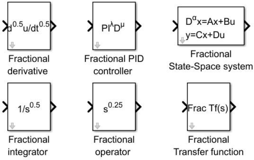
Compered to Labview, MATLAB has a wider range of available tools. In MATLAB’s add-ons library there are some easy-to-use toolboxes, which provide complete structures and functions for fractional calculus and control, based on different definitions or approximations. Among them, the most extensive can be distinguished: the FOMCON toolbox [28, 29, 30, 31], FOTF toolbox [32] and Ninteger toolbox [33]. The FOMCON toolbox is the most complex available tools as of today, it includes many useful easy-to-use blocks such as complete FOPID Controller, fractional integrator/derivative, fractional transfer function both in continues and discrete-time domain and many more. FOMCON can be used for design, analysis, simulation and control of fractional-order systems. The fractional-order elements are approximated using Oustaloup’s recursive filters, described in Section 3.2. It also comes with controller tuning under performance and robustness specifications. However, its most significant advantage lies in providing a comprehensive, end-to-end framework that facilitates the seamless transition from fractional-order system model to a fully implementable control solution. FOTF toolbox is less complex than FOMCON but still provides all the basic blocks; fractional operator, Caputo operator, Riemann-Liouville operator, FOPID Controller and FOTF Model.
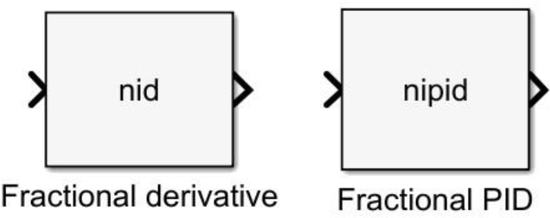
The Ninteger toolbox has a wide range of available functions with focus on CRONE Controllers and approximations but comes with only two universal block structures: Fractional derivative and FOPID controller. Figures 4.1, 4.2 and 4.3 show examples of universal blocks from the mentioned toolboxes. Those toolboxes are also suitable for hardware implementation.

. Real-Time implementation
For real-time implementation of fractional-order algorithms, a number of tools can be highlighted. There are MATLAB libraries such as HDL Coder for DAQ boards with FPGA modules or FPGA and ASIC standalone systems and PLC Coder for PLC controllers. Both of those libraries are toolsets to automatically generate code from the simulink graphical interface for a particular target, for example, VHDL/Verilog for FPGAs and ST and Ladder Logic for PLCs, and allow verification of code operation, as well as providing support for external interfaces. However, these libraries support a limited number of hardware platforms, so one must verify compatibility with specific hardware before deciding to use them.
There is also third-party software interfacing with MATLAB available commercially, such as QUARC and dSPACE real-time software. These software solve the problem of handling embedded systems as a target and support the design and implementation of complex algorithms. Together with the software, it is possible to use dedicated measurement boards so that all control and measurements can be performed by a single unit fully compatible with Simulink. Within the scope of this work, the QUARC software kit was used together with a measurement board with an FPGA module, acting as an external target in the form of NI-myRIO-1900. Most of the measurement boards from National Instruments are compatible with the QUARC software; hence, the NI-PCI-6221 card could also be used. It is worth mentioning that the previously presented equation describing the FOPID controller (eq. (3.1)) in the case of practical implementation often requires consideration of saturation and anti-windup algorithms.
FRACTANCE DEVICES
A device demonstrating behavior governed by fractional-order dynamics is termed a fractance [34, 35]. The fractance devices can be classified by three basic types: domino ladder circuit network, a tree structure of electrical elements and net-grid network. Each is built with infinitely many resistors R and capacitors C connected in series or parallel. As part of the study, it was decided to consider the case of a domino ladder system described as a Cauer type I structure, shown in Figure 5.1. Since there is no phenomenon of infinity in reality, a fractance with dynamics corresponding to a non-integer order α system, can be approximated by finite number of elements using truncated continued fraction expansion (CFE). Using the aforementioned CFE method, the impedance of domino ladder system can be described as: [34]
where, Cα - is pseudo-capacity of the system, Rn is resistance value and Cn is capacitance value. The circuit RCα in Figure 5.1, can be described using Kirchhoff’s second law as: where uR(t) is voltage of resistor R, uin(t) is source voltage e and uout(t) = V0–V– is voltage on the fractional-order element.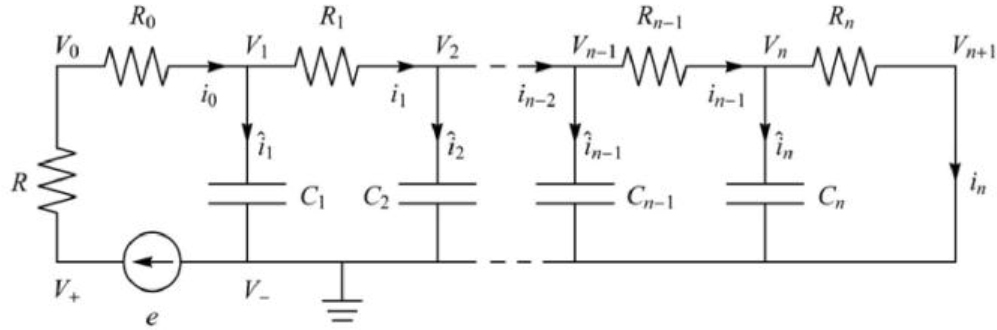
Considering that
equation eq. (5.2) can be expressed as which can then be converted to after applying the Laplace transform, the following was obtainedSIMULATION ANALYSIS
. Toolbox comparison
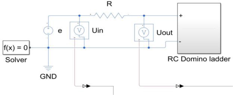
The domino ladder system from Figure 5.1 was recreated in Simulink using values specified in [34] for α = 0.60 with Simscape electrical library as shown in Figure 6.1. That is because such system can effectively be used as a base sample for comparison with models created with considered toolboxes.
Using eq. (5.6) and FOMCON, FOTF and NINTEGER Toolboxes several models were created with approximation order of 5 and frequency range [0.001;1000]. All of the considered models were then supplied with a voltage step signal of 10 V and their response was compared with domino ladder system response. This step is essential to verify that all fractional integrators provided by the toolboxes perform as expected and to identify the most suitable implementation before applying them in control scenarios. The responses of those models are shown in Figure 6.2, where the difference between them is apparent, but appears to be insignificant.
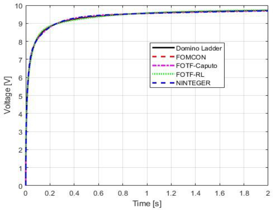
Hence, in addition, a correlation showing the relative error between the responses of the models and the domino ladder system over time was determined, which can be seen in Figure 6.3.
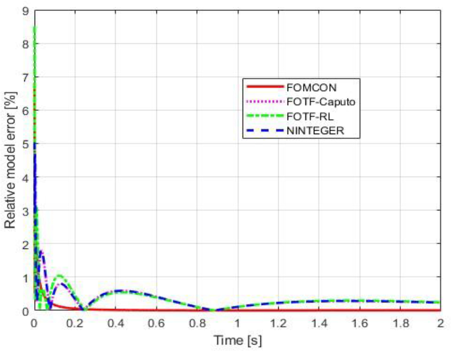
Analyzing the results shown in Figure 6.3, it turns out that the best approximation of the non-integer-order element was obtained for the FOMCON toolbox. Therefore, FOMCON Toolbox will be used for simulation and practical implementation.
. Second order system
Now an example implementation of a fractional-order algorithm using the aforementioned tools will be presented, where a very simple system without delays will be taken as the control plant in order to show the required operations. Note, however, that in reality many systems have delays, but the approach will remain the same. Now let’s consider second-order control plant which can be described as
When K = 1, T1 = 1.5 and T2 = 2.5 the transfer function eq. (6.1) of plant takes form
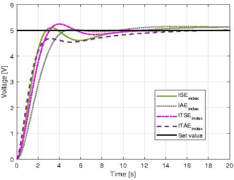
Based on equation (6.2), a simulation was carried out using both PID and FOPID controllers, where each controller was implemented according to equation (3.1). For the PID controller, the parameters were set to λ = 1 and μ = 1, while for the FOPID controller, the values were selected within the fractional ranges λ ∈ (0,1) and μ ∈ (0,1).
As for the tuning method, Modified Grey Wolf Optimization algorithm [18, 36] was implemented and both controllers were tuned with the same conditions and constraints. The key distinction lies in the number of optimized parameters: the PID controller required tuning of three parameters (kp, ki, kd), whereas the FOPID controller involved five parameters (kp, ki, kd, λ, μ).The cost function eq. (6.3) consisted of the cost of deviation (CF_E) and the cost of control (CF_U) with weights of 400:20. Considering the control effort in the optimization process helps to obtain controller settings that can be realistically implemented in hardware, as the resulting control signal stays within the limits supported by the measurement card, e.g. ±10V. The cost of deviation can be determined using different integral indices: ISE, IAE, ITSE or ITAE, while the cost of control was determined as the square of the error. Depending on the selected performance index, the optimization algorithm emphasizes different characteristics of the system response. Therefore, a separate controller tuning procedure was performed for each of the specified indices to examine how the choice of a particular criterion influences the final outcome of the algorithm. The algorithm yielded four sets of settings for the PID and FOPID controller, using the aforementioned indices, 40 iterations and 20 searching agents. It is important that the optimization process is carried out for a higher setpoint than the one envisaged in the target implementation. The closed-loop response of the system (6.2) with FOPID control is shown in Figure 6.4. The ITSE criterion provided the best performance, and thus its associated controller settings were adopted for implementation. The cycle execution time was 0.002 s for both controllers.
HARDWARE IMPLEMENTATION
. Implementation procedure
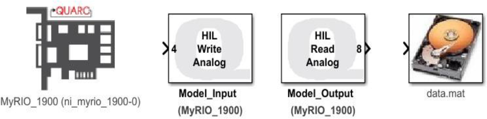
The hardware unit supporting the control algorithm is a measurement board NI-myRIO-1900. Its operation and control have been implemented using QUARC software, which provides the blocks shown in Figure 7.1. The first of these (HIL Initialize) is the hardware configuration block, where all the parameters of the system are specified, including the number of inputs/outputs and their channel numbers, measurement ranges, encoder inputs, etc. Further on, you can see the analog input and output blocks of the card, as well as the block that allows you to save data to a file (To Host File). Analog laboratory model was used to simulate the operation of the system eq. (6.2).
The process of implementing the algorithm from Section 6.2. into a real system is shown in Figure 7.2. The first three steps are associated with Matlab Simulink software, while the next four are implemented by the QUARC add-on.
Modeling in Simulink – design the chosen control algorithm, in this case a PID/FOPID controller in Simulink. It is important to use blocks from the QUARC library, from Figure 4.1 and Figure 7.1. Remember to define the I/O along with the board configuration via the HIL Initialize block.
FOPID Tuning – input the designated controller settings – kp, ki, kd, λ, μ.
Discretization – as the algorithm is ultimately intended for a real system, it should be discretized with sample time Ts. In this case, Ts was taken as 0.002s.
C/C++ Code Generation – compile the discretized model to C/C++ using QUARC’s auto-code tools.
ARM Target Adaptation – modify generated code for ARM architecture compatibility (e.g., myRIO-1900).
Deployment to Real-Time System – upload the executable to the myRIO-1900 real-time target.
Performance Verification – validate real-time operation against design requirements (e.g., step response, stability).
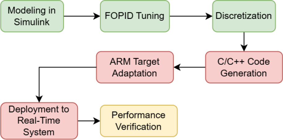
It is critical to select the correct target type in the QUARC compiler options during the initial model preparation stage (Step 1), as Steps 4–6 are automatically executed by QUARC during compilation based on the specified target. For this implementation, the quarc_linux_rt_armv7 target was chosen, as it provides a generic real-time framework for ARM-based systems, including the myRIO-1900 board.
Due to the interferences introduced by the control plant, a low-pass filter described as eq. (7.1), was applied to its output to negate its effect on system operation.
. Experimental Results
The system from section 6.2 has been implemented with a procedure from Figure 7.2. into myRIO-1900 using the PID and FOPID controller parameters optimized for the ITSE criterion. Figure 7.3 presents the closed-loop responses of both the physical plant and simulated system, while Figure 7.4 displays their corresponding control signals.
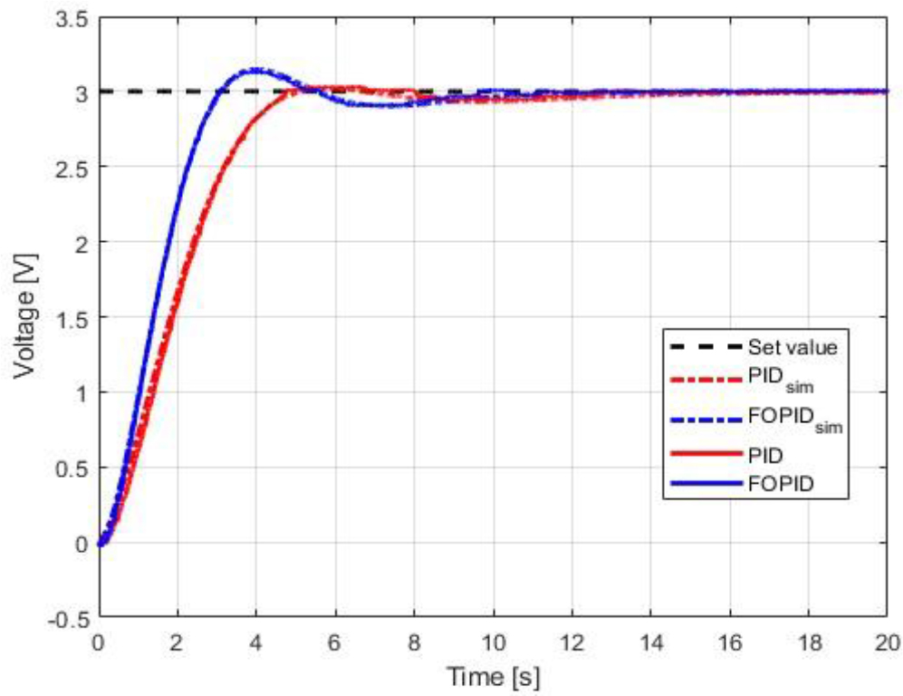
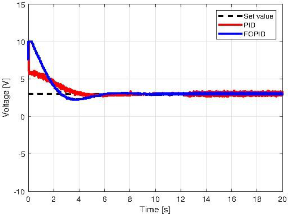
Analyzing the results shown in Figures 7.3 and 7.4, it is evident that the experimental results coincided with the simulation results. The values of the cost function obtained in both the simulation and the experiment, along with the selected values of the controller settings, are summarized in Table 1. Clearly the FOPID controller scored about 30% better in terms of control deviation and about 6% better in terms of control cost than the PID controller in both the simulations and the experiment. The FOPID controller demonstrated superior performance with a 16% lower RMSE (Root Mean Square Error) value compared to the conventional PID controller, further validating its effectiveness for the given control application. The experimental results also yielded better results in terms of control deviation than the simulation with comparable value of control signal. In addition, in the waveform of the control signal in Figure 7.4, it can be seen that the FOPID Controller handled the control signal better. It is also worth mentioning that control signal from FOPID controller was more resistant to interference than PID controller, which is visible in Figure 7.4.
CONCLUDING REMARKS
In this paper, a method for design and implementation of fractional-order controller for both simulation and experiment were presented. The analysis of currently existing solutions made it possible to identify current trends in the tuning of FO controllers and showed the superiority and potential of FOPID controllers over their classical counterparts. The available tools for working with fractional-order calculus were presented, and the FOMCON Toolbox was clearly identified as the current best solution. Then the physical implementation of the fractional-order element is shown, along with an example implementation procedure for a given model of a control object. It turns out that the process of tuning FOPID controllers is relatively lengthy and requires appropriate definition of search ranges and cost functions to enable a smooth transition from the simulation environment to the real one. The solution shown can also be easily applied to other control objects and hardware platforms. Further research will focus on switched systems, which will eventually be enriched with fractional-order controllers.