1. INTRODUCTION

Numerous engineering systems experience unwanted vibrations. Managing these vibrations in mechanical systems poses significant challenges, requiring methods to either eliminate or reduce them. In the field of civil engineering, structures were traditionally designed without considering the impact of soil-structure interaction (SSI), assuming it to be negligible. However, it has been demonstrated that various factors influence the SSI phenomenon's outcomes. Various approaches exist to address the SSI effect, one of which involves utilizing the substructure method. This technique relies on superimposing two substructures (soil and structure), assuming a rigid interface between them.

Control is the name given to the task to arrive to a desired result. It is applied to structures of civil engineer offer a protection against the harmful effects of the destructive seismic force or discomfort of the man on the movement structural induced by the strong wind and other types of vibrations. Structural control is defined like a mechanical system installed in a structure to reduce the structural vibrations during the loadings such as the winds, eathquakes…etc. It is developed by Yao 1972, Soong 1990, Housner et al. 1997, Spencer and Nagarajaiah 2003.

Into paraseismic structural control is defined like a new fashion of prootection [1], which this time does not propose any more to absorb the enrgy of an earthquake by a reinforcement of the structure itself, in order to make it resistant, but by the addition of special devces aiming to contain or control the answer of the structure at the time of the arrival of a seismic wave by the soil. Also let us note that some of these monitoring systems of the answer, are used to protect from the structure against of another risks that the seismic risk, such as the wind, of the risks of to special equipment.

Several studies ignore the effect of soil-structure interaction (SSI) in the study of reliability and effectiveness of control on seismic response. To verify the effect of SSI on the efficiency and reliability of soil control, Wang et al treat the effect of passive TMD on the simic response of a long building with soil-structure interaction, the results show that the passive TMD will become poorly tuned when the SSI effect is introduced with different ground models [2]. To solve the problem, a adaptive-passive eddy current pendulum Tuned Mass Damper (APEC-PTMD) was developed [3–4], an APEC-PTMD is applied to a 40-story building including SSI, and four different soil conditions are considered, the results show that the APEC-PTMD gives better seismic protection than the passive TMD in the case of a structure with the SSI [2]. Which concludes that we must take into consideration the effect of the ISS on the effect of the control on the seismic response of the structures. This structural monitoring system can be divided into two parts, a part relates to the algorithms of control [5–6]. In this article one with used actice control and algorithm GOAC. Our second objective in this study is to introduce the effect of the soil-structure interaction by the substructure method cited in [5].

2. CONTROL STRUCTURAL

In recent years, increased attention has been paid to the in-depth study of various types of control systems, with the aim of improving their effectiveness and resilience to natural hazards such as earthquakes and hurricanes. Depending on the energy and performance levels required, these systems can be classified into four distinct categories: passive, active, semi-active and hybrid control systems [7].

A passive control system is a system in which structural vibrations are reduced by a device, which gives force to the structure in response to its movement. Passive monitoring has certain advantages. First, it does not require an external power source for its operation, which makes it more economical than other systems. In addition, it is smaller in size requiring less space for its installation. Finally, due to its simplicity, this type of control has received a lot of attention from researchers, making it more reliable to use. The principle of this system is the integration of materials or systems, possessing damping properties, and therefore the structural vibration dampened passively [8–9].

The most common in this type are seismic isolation and tuned mass damper (TMD) [10–11]. Seismic isolation is a seismic design approach that relies on decoupling ground motion from that of the structure, resulting in a reduction in the forces applied to the structure during an earthquake. The first experiments with the principle of seismic isolation date back to the beginning of the 20th century, and the first application of modern seismic isolation technology was carried out in 1969 [12].

A tuned mass damper (TMD) is a device consisting of a mass, a spring, and a damper that is attached to a structure in order to reduce its dynamic response. The frequency of the damper is tuned to a particular structural frequency so that when that frequency is excited, the damper will resonate out of phase with the structural movement. When it is poorly tuned, the effectiveness of the control will be rapidely diminished [13–14]. An active control system is a system that is fully adaptive and uses an external power supply to produce the required control force to decrease structural response [8]. The advantage of an active control system is that the system achieves an excellent control result. However, there are downsides. It is an expensive system to design and expensive to use because of its high power requirement. In addition, it tends to take up more space than passive controls [8].

In the semi-active control system, mechanisms are employed to control or assist a passive control device. The inherent advantage of a semi-active control device is that the mechanism used does not require a large amount of external power. Many semi-active devices can be powered by batteries protecting them against sudden loss of power during earthquakes. In addition, semi-active control devices are mechanically less complex than active devices. Semi-active systems are more aggressive than passive systems and usually obtain control results close to that of an active control system [8].

The semi-active control strategy is similar to the active control strategy [15]. Only here, the control system does not add energy to the structure. Several research studies have carried out on the effect of semi-active control on the attenuation of the seismic response [16–17, 13, 1, 10–11].

Semi-active devices require much less power than active devices; and energy can often be stored locally, in a battery, thus making the unit type semi active independent of any external power supply. Another critical theme with active control is stability robustness with respect to sensor failure; this problem is particularly difficult when centralized controllers are employed [18].

There are many semi-active systems that can be fitted to structures of any type. They are also used to meet needs other than response control in the field of earthquake architecture [5].

The most common in semi-active systems are magneto-rheological fluid dampers [19], these are dissipative non-linear components, used in semi-active suspension control, where the damping coefficient varies according to the electric current. The hardness of this type of shock absorber depends on the viscosity of the fluid, which is controlled by the magnetic field. This system with a Magneto-rheological fluid inside, is a silicone oil containing ferromagnetic particles of micrometric size forming aggregated structures under the action of a magnetic field [20]. Wall et al. [16] suggest the integration of a semi-active tuned mass damper (STMD) to enhance the seismic resilience of base-isolated structures. They concluded that the STMD significantly improves the displacement and acceleration capabilities of these structures, irrespective of their linearity.

Hybrid control strategies have been studied by many researchers to exploit their potential to increase the reliability and overall efficiency of the actively controlled structure [21]. These hybrid control systems have received a lot of attention since the 1990s [22]. A hybrid control system generally refers to a combined passive and active control system, which increases the reliability and overall efficiency of the potentially controlled structure [23]. So this system wins the advantages of both techniques. This makes this system capable of halving the amplitude of movement of constructions [5]. An example of a hybrid system, a Hybrid Mass Damper (HMD) is a system proposed to suppress the response of a large building against strong winds and moderate seismic loads to meet the requirement on the vibration level for comfort [24].

3. SOIL STRUCTURE INTERACTION

Soil structure interaction is often neglected by engineers when analyzing and designing a structure, although this phenomenon has a great effect on the behavior of structures, which depends on the characteristics of the soil and structure. herself. For this reason, several researches have been done in this area. We will briefly cite a few:

In 1996, Steven L Kramer [25] presented in “Geotechnical EQ Engineering” the effects of the soil structure interaction phenomenon, and gave different methods to take into account the SSI effect. The SSI problem was treated in 2000 in the context of multi-support structures, such as the bridge, by Claugh & Penzien in their work “Dynamics of structures”.

A modeling is made in finite elements (2D) of the dynamic soil-structure interaction of a building by the substructure method, in 2000 by M. Kutanis & M. Elmas [26]. Several comparisons were carried out:

In 2004, John P. Wolf & Andrew J. Deeks [27] developed the theory of cones (conical column-beams), who applied it to foundation vibration analyses. This work shows the influence of soil characteristics on the movement of the structure.

Also in 2004, H. Shakibet and A. Fuladgar [28] formulated an approach in the temporal domain for the 3D linear analysis of the ground-structure interaction of a building with an anti-symmetrical shape, for the evaluation of the seismic response of the structure. The contact between the foundation and the ground is modeled by linear plane interface elements of zero thickness.

In 2005, M. Oudjeneet al [29] demonstrated that the modification of the seismic action of high frequencies is not taken into account by the shape of the different response spectra thus proposed in the high frequency range. Then, they discussed the current state of these computational spectra and suggested that the lengthening of the fundamental period does not systematically imply the decrease of the spectral acceleration.

In the seismic calculation of structures, the excitation is defined by one or more acceleration recordings often measured at the ground surface in the absence of any construction. These recordings give the free-field accelerograms. In the presence of a building or any other construction, the movements in the vicinity of the foundations may differ from those existing in the open field. Indeed, the forces in contact between the structure and its foundation disrupt the movement of the ground, and the moment of embedding at the base causes its rotation. This phenomenon is referred to as “Soil Structure Interaction” or “SSI” [30].

There are many methods to take into account the effect of soil structure interaction. Many studies have been conducted to demonstrate a detailed comparison between approaches to soil-structure interaction (SSI) analysis, such as direct and indirect methods (substructure), etc. [31,32,33,34,35]. The direct method is considered the most rigorous approach for solving SSI problems for complex structural geometries and the nonlinearity of soil; in this approach, the structure and soil are modeled as a single system [36].

While this strategy is highly effective for solving simple linear and difficult nonlinear problems, it is also complicated, inefficient, and expensive, making it an illogical way to design typical structures [37]. The substructure method is widely used in current SSI analysis practice due to its simplicity and computational efficiency [31, 35]; many researchers have adopted this approach for soil-structure interaction analysis [32,33,34]. However, researchers have discussed the limitations of this approach. Therefore, Taha A. et al [31] suggest future research to develop this approach to enhance the accuracy of substructure approach simulation.

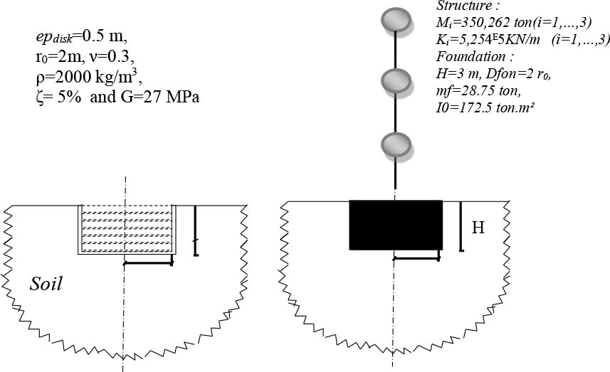
We will use the substructure method. This method is based on the principle of the superposition of two substructures (soil and structure), such that the soil-structure interface is assumed to be rigid (see Fig. 1).

Fig. 1.

The two substructures : soil and rigid structure with soil-structure interface [38]

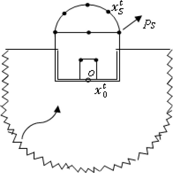
The loads can be applied to the structure, or through the soil by seismic excitation which propagates vertically in the form of waves, applied to the soil structure interface [38].

The node at the center of the soil-structure interface is designated by 0, and the other nodes of the structure are designated by S.

The equation of motion in the time domain expresses the system equilibrium, which gives :

In the complex domain we have :

Equation (1) in the complex domain becomes :

We can write equation (4) in the form :

The dynamic stiffness matrix [S(w)] is

Equation (5) becomes :

Such that [G(w)] is the dynamic flexibility matrix of the system.

The equation of motion (5) of the structure is formulated as follows [38] :

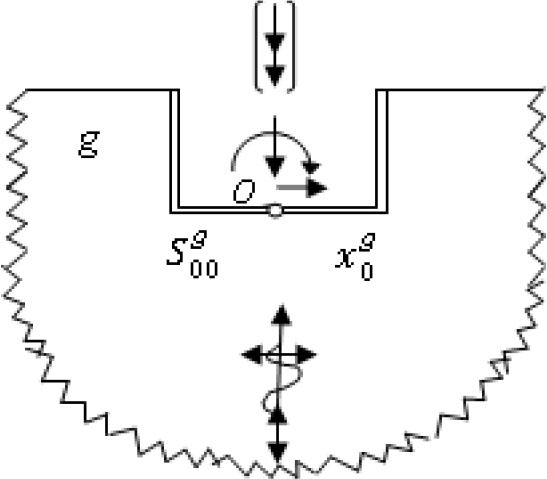
The substructure of the unbounded ground system, with a rigid and massless ground-structure interface is discussed, to express {P₀(w)}, this system is illustrated in Fig. 2 [38].

Fig. 2.

Substructures: unbounded soil

As [S00g(w)] denotes the dynamic stiffness matrix, and {x0g(w)} represents the displacement amplitudes of the soil system mass caused by seismic excitation [38].

For P-waves to propagate vertically, the free-field displacement is also vertical, and the effective base input motion consists of a vertical component, which could result in free-field displacement in the fixed zone. Conversely, for S-waves, the free-field displacement is horizontal, and the base input motion consists of a horizontal component, leading to an average free-field displacement and rotation in the fixed zone. For the motion {x0g(w)} , the interaction forces acting on node 0 vanish, because for this loading condition, the soil-structure interface is a free surface. This implies that the soil interaction forces depend on the position relative to the effective base input motion {x0g(w)} , and their amplitudes can be expressed as follows [38]:

From equation (9), equation (8) can be reformulated as follows

Equation (10) represents the motion equation of the soil-structure system with a rigid soil-structure interface expressed in terms of total displacement amplitudes [38].

4. EQUATION OF STATE OF A STRUCTURE OF TYPE BEAM-COLUMN WITH AND WITHOUT INTERACTION CONTROLLED BY AN ACTVE TENDON

With SSI

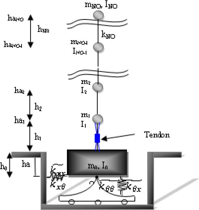
For the develpoment of th equation of mtion, one considers a structure beam-column in “NO” floors controlled actively by active tendons (Fig. 3). To take account of the soil-structure interaction, it is supposed that the structure rests on a flexible foundation built-in a soil with several in depht layers whose characteristics can vary from a layer with another but ramain constant along the layer considered. In this case the effect of the soil will be repesented by forces of ineractions noted R0(t).

(11)

[M]{X¨tg(n)}+[C]{X˙tg(n)}+[K]{Xtg(n)}={δ}x¨0g(n)+[γ]{U→(n)}+{0−R0(n)}

Fig. 3.

Model of a structure equipped with active tendons and with SSI

By separating the degrees of freedom from the structure and those of the foundation, the equation (11) will be written [39]:

(12)

[[MSS]NO×NO[MS0]NO×2[M0S]2×NO[M00]2×2]{x¨stg(n)x¨0tg(n)}+[[CSS]NO×NO[CS0]NO×2[C0S]2×NO[C00]2×2]{x˙stg(n)x˙0tg(n)}+[[KSS]NO×NO[KS0]NO×2[K0S]2×NO[K00]2×2+[K˜]2×2]{xstg(n)x0tg(n)}={δSδ0}x¨0g(n)+[[γS]NO×NCR[γ0]2×NCR]{U→(n)}+{0−R0(n)}

Where the matrices [M_SS], [C_SS] and [K_SS] represent the respective diagonal masses of the floors, the proportional damping matrix, and the stiffness of the symmetric columns of the structure. The matrices [M_S0], [C_S0] and [K_S0], as well as the matrices [M_0S], [C_0S] and [K_0S], respectively, denote the mass, stiffness, and damping matrices associated with the superstructure and the rigid foundation. The matrices [M₀₀], [C₀₀] and [K₀₀] respectively represent the mass, stiffness, and damping associated with the rigid foundation.

The vector {δ_S} represents the vector of horizontal acceleration coefficients of the soil for the superstructure. The vector {δ₀} represents the vector of horizontal acceleration coefficients of the soil for the foundation.

The matrices [γ_S] and [γ₀] represent the localization matrices of the controllers for the superstructure and the foundation, where NCR is the number of active controllers.

{Xstg(n)} , with dimensions (NO×1), represents the vector of floor displacements (xNOtgxNO−1tg … xitg … x2tgx1tg)T and {X0tg(n)} , with dimensions (2×1), is the vector of displacement and rotation of the foundation at point “O” (x0tg,θ0tg)T .

The vector {R₀(n)}=[R_x(n)R_θ(n)]^T, with dimensions (2×1), where R_x(n) is the horizontal interaction force and R_θ(t) is the interaction moment at point 0.

To solve this system, it is assumed that the state vector Z^tg(n), with dimensions (2(NO+2)×1) [1] :

(13)

Ztg(n)={{xstg(n)}{x0tg(n)}{x˙stg(n)}{x˙0tg(n)}}

In replacing equation (13) into (12), we obtain the following state equation [39]:

(14)

{Z˙tg(n)}=[A]{Ztg(n)}+[B]{U→(n)}+{E(n)}

We can express equation (14) in the following form :

(15)

{Z˙tg(n)}=[D]{Ztg(n)}+{E(n)}

Where [D] is the time-independent 'plant' matrix, with dimensions of (2(NO+2) x 2(NO+2)):

(16)

[D]=[A]+[B][GISS]

With: [G^ISS] The control gain matrix, computed in this work using the Generalized Optimal Active Control (GOAC) algorithm (section 4.1.1) [40].

[A] is the characteristic matrix of the controlled system, with dimensions of (2(NO+2) ×2(NO+2)) :

(17)

[A]=[[0][I]−[[M]−1[K]]−[[M]−1[C]]]

[B] is the actuator placement matrix, with dimensions of (2(NO+2) × NCR)

(18)

[B]=[[0][M]−1[γ]]

{E} is the vector of external disturbances, with dimensions of (2(NO+2) × 1), {C} is the vector related to the base acceleration of the structure, with dimensions of (2(NO+2) × 1), {Ř₀(n)} is the vector of accelerations, with dimensions of (2(NO+2) × 1), and {R̃₀} is the dynamic vector of equivalent forces.

The vectors {x0tg(t)} and {R₀(t)} at time t are related by the system's ground flexibility matrix through the following convolution integral [40] :

(19)

{x0tg(t)}=∫0∞[F00g(τ)]{R0(t−τ)}dτ

With: [F00g(τ)] is the dynamic soil flexibility matrix.

Where [F00g(w)]=[S00g(w)]−1 , where [S00g(w)] is the dynamic soil stiffness matrix

Generalized Optimal Active Control (GOAC) algorithm

Research efforts in active structural control have focused on various control algorithms based on multiple control design criteria. These active control algorithms are used to determine the control force of the measured structural response, providing a control law and a mathematical model of the controller for an active control system [39]. Some are considered classical as they are direct applications of modern control theory [41]. Examples include the Riccati Optimal Active Control (ROAC) based on integrated performance over the entire duration of seismic excitation, and the classic pole placement algorithm, showing promising application in civil engineering smart structures [39]. These classical algorithms, however, are not truly optimal as they ignore the excitation term in their calculation [41]. Recognizing that at any particular time t, knowledge of the external excitation may be available, this knowledge can be used to develop improved control algorithms [41]. This led to the development of the Instantaneous Optimal Active Control (IOAC) algorithm, which differs from ROAC in that its performance index depends on time [39]. However, IOAC's control force is proportional to the time increment, resulting in non-uniform control forces for structures subjected to different seismic loadings over time [39]. To address these limitations, Japanese researchers Cheng and Tian developed the Generalized Optimal Active Control (GOAC) algorithm, which can adjust the feedback gain matrix to achieve better controllability [39–40].

The following equation is the simplest notation of equation (14) :

(20)

{Z˙(t)}=[A]{Z(t)}+[B][U→(t)]+{E(t)}

All parameters in the following algorithms pertain to a building taking into account the effect of soil-structure interaction. In this section, we will examine in detail the GOAC algorithm for closed-loop structural control [39].

– The transversality conditions:

Let's consider a system governed by free-end boundary conditions with equation (20) given by [40] :

(21)

{ti−1=t0+(i−1)Δt{Z(ti−1)}={Zi−1}ti=t0+(i)Δt

Such as :

Δt=1N(tf−t0);   i=1,2,…,N

{Z_i−1} : is the value of {Z(t)} a t_i−1, vector of dimension (2(NO+2)×2(NO+2))

Equation (21) can be written in the following vector form :

(22)

{Ω}={Ω1{Ω2}Ω3}={(ti−1−t0)−(i−1)Δt{Z(ti−1)}−{Zi−1}(ti−t0)−(i)Δt}={0}

By introducing multipliers {μ} and {λ(t)} and forming :

(23)

G=g({Z(ti)})+{μ}T{Ω}

(24)

F=f¯(t)−{λ(t)}T{f(t)}

Such as :

(25)

g({Z(ti)})=12{Z(ti)}T[S]{Z(ti)}

(26)

f¯(t)={Z(t)}T[Q]{Z(t)}+{U(t)}T[R]{U(t)}

(27)

{f(t)}=12([A]{Z(t)}+[B]{U(t)}+{E(t)}−{Z˙(t)})

Then the transversality condition can be expressed as follows

(28)

dG−[({∂F∂{Z˙(t)}}T{Z˙(t)}−F)dt ]ti−1ti+[{∂F∂{Z˙(t)}}Td{Z(t)}]ti−1ti=0

Applying equation (28) to equation (23) and (24), we obtain :

(29)

[S]{Z(ti)}−{λ(ti)}={0}

Where : g({Z(t_i)}) is an optimization function of boundary conditions at each end time t_i.

[S] and [Q] are positive semi-definite matrices, both of dimension (2(NO+2) × 2(NO+2)). [R] is a positive definite matrix of dimension (NCR × NCR).

– Generalized performance index:

In this algorithm, the control time interval [t₀, t_f] is divided into N segments in the calculation of the performance index J, which is defined and minimized to obtain an optimal solution for the state vector {Z(t)} and the control force vector {U(t)} [1].

(30)

J=∑i−1n12∫ti−1ti({Z(t)}T[Q]{Z(t)}+{U(t)}T[R]{U(t)})dt

The boundary conditions in the performance index equation in the Riccati algorithm are as follows :

(31)

{{Z(t0)}={Z(tf)}={0}{U(t0)}={U(tf)}={0}

The performance index J will be integrated step by step. At each integration step of [t_i−1, t_i] such that (i =1, 2, ..., N), at least one of the two limit values of the state vector is unknown . The values of the state vector {Z(t)} is specified at t_i−1, and unspecified and mobile at time t_i.

We have already said that the state vector {Z(t_i)} is unknown, it must be reduced to a minimum to include it in the performance index equation. By introducing the transverse conditions at time t_f, the performance index is expressed as follows:

(32)

Ji=g({Z(ti)})+12∫ti−1ti({Z(t)}T[Q]{Z(t)}+{U(t)}T[R]{U(t)})dt

Thus :

(33)

Ji=g({Z(ti)})+12∫ti−1tif¯(t)dt

– The feedback gain matrix and the control force.

The Euler equations :

(34)

{∂F(t)∂{Z(t)}−ddt(∂F(t)∂{Z˙(t)})={0}∂F(t)∂{U(t)}−ddt(∂F(t)∂{U˙(t)})={0}

Replacing equation (24) into equation (34), we will have :

(35)

{∂∂{Z(t)}[12{Z(t)}T[Q]{Z(t)}]=[Q]{Z(t)}∂∂{Z(t)}[{λ(t)}T[A]{Z(t)}]=[A]T{Z(t)}ddt[∂∂{Z˙(t)}(−{λ(t)}T{Z˙(t)})]=−{λ˙(t)}∂∂{U(t)}({U(t)}T[R]{U(t)})=[R]{U(t)}∂∂{U(t)}({λ(t)}T[B]{U(t)})=[B]T{λ(t)}

So equation (34) becomes :

(36)

{[Q]{Z(t)}+[A]T{λ(t)}+{λ˙(t)}={0}[R]{U(t)}+[B]T{λ(t)}={0}

By replacing equations (25) and (22) into equation (23), we find the function G :

(37)

G=12{Z(ti)}T[S]{Z(ti)}+μ1[(ti−1−t0)−(i−1)Δt]+{μ2}T[{Z(ti−1)}−{Zi−1}]+μ3[(ti−t0)−(i)Δt]

Where G is the augmented function of the function g.

As the multiplier {μ}^T=[μ₁, {μ₂}^T, μ₃]

With:

(38)

{∂G∂ti−1=μ1∂G∂{Z(ti−1)}={μ2}∂G∂ti=μ3{∂G∂{z(ti)}}=[S]{Z(ti)}

From the second equation of equation (36), we have the equation of the control force :

(39)

{U(t)}=−[R]−1[B]T{λ(t)}=⇒

(40)

{U(t)}=−[R]−1[B]T[S]{Z(t)}

(41)

{U(t)}=[GJSS]{Z(t)}

So :

(42)

[GJSS]=−[R]−1[B]T[S]

So, where [G] is the feedback gain matrix, this matrix represents an optimal control law. It is of dimension (NCR × 2(NO+2)). It is independent of time t, where t ∈[t_i−1, t_i] and of the time increment Δt.

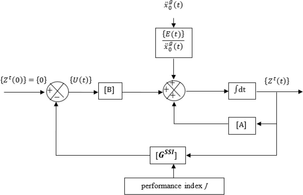
From equation (42), we notice that if we choose the matrix [S]=[P], where [P] is the Riccati matrix, we obtain the same equation for the feedback gain matrix found in the Riccati algorithm. This means that the Riccati algorithm is a case of the GOAC algorithm, which is why the algorithm is called the generalized GOAC algorithm. This gain matrix [G^ISS] is obtained from the state equation (20), which can be solved using the diagram in the following figure.

Fig. 4.

Flowchart of solving the state equation with active control [18]

In the case of SSI, the matrices [S] and [Q] are of dimension (2(NO+2) × 2(NO+2)). The matrix [R] is of dimension (NCR × NCR). They are defined as follows :

(43)

[Q]=[[KSS][KS0][0][0][KS0]T[Ǩ00][0][0][0][0][MSS][0][0][0][0][M00]]

And

(44)

[R]=[[γS][γ0]][[KSS][KS0][KS0]T[Ǩ00]]−1[[γS][γ0]]

With:

(45)

[Ǩ00]=[k1+Kxx˜−ha1k1+Kxθ˜−ha1k1+Kθx˜ha12k1+Kθθ˜]−1

The matrix [S] is chosen as an arbitrary row matrix :

(46)

[S]=[[0][0][SD][SV]]

To ensure a semi-definite positive state of the matrix [S], the symmetric matrix can be chosen as follows:

(47)

[S]=γD[ΩV−1[Ǩ][Ǩ][Ǩ]ΩV[Ǩ]]

With :

(48)

[Ǩ]=[[Kss][Ks0][KS0]T[Ǩ00]]

Where γ_D is the stiffness scale factor, and Ω_V is the damping scale factor.

We can write equation (14) as follows:

(49)

{Z˙tg(t)}=[D]{Ztg(t)}+{E(t)}

Where [D] is the matrix of the horizontal component of the damping force, and it is of dimension (2(NO+2) x 2(NO+2)) :

(50)

[D]=[A]+[B][GISS]

{E} is the vector of external disturbances, it has dimension (2(NO+2) x 1)

(51)

{E(t)}={C}x¨0g(t)+{−Ř0(t−Δt)}

The influence of S_D, S_V, γ_D and Ω_V on the overall system can be studied by substituting the equation for the gain matrix from equation (42) into the equation for the matrix of the horizontal component of the damping force (50), yielding:

(52)

[D]=[A]−1R[B][B]T[S]

The technical solution:

(53)

[U→(t)]=[GSSI]{Zt(t)}

[G_SSI] is the feedback gain matrix, it is time-independent, and it has dimensions of (NCR x 2(NO+2)).

The simplification of equation (20) is as follows :

(54)

{Z˙(t)}=[D]{Z(t)}+{E(t)}

(55)

[T]=[{a1}{b1};…;{ai}{bi};…;{aNO+2}{bNO+2}]

The transformation matrix [T] is constructed from the eigenvectors of the matrix [A]. It is necessary to transform the equation of state into canonical form. In which {a_i} and {b_i} are respectively the real and imaginary parts of the eigenvector i of the matrix [A], and they have dimensions (2(NO+2) x 1). So the transformation matrix [T] has dimension (2(NO+2) x 2(NO+2)).

(56)

[Λ]=[T]−1[D][T]

[Λ] is a real matrix, it has dimension (2(NO+2) x 2(NO+2)), and it has the following form :

(57)

[Λ]=[[Λ1]⋯[0]⋯[0]⋮⋱⋯⋯⋯[0]⋮[Λi]⋯[0]⋮⋮⋮⋱⋯[0]⋮[0]⋮[ΛNO+2]]

With :

(58)

[Λi]=[μivi−viμi]

The solution to equation (54) is expressed as follows:

(59)

{Z(t)}=[T]{Φ(t)}

Substituting equations (56) and (59) into (54), we obtain:

(60)

[T]{Φ˙(t)}=[D][T]{Φ(t)}+{E(t)}

(61)

{Φ˙(t)}=[T]−1[D][T]{Φ(t)}+[T]−1{E(t)}

(62)

{Φ˙(t)}=[Λ]{Φ(t)}+{Γ(t)}

With :

(63)

{Γ(t)}=[T]−1{E(t)}

(64)

{Z(0)}={0}⇒{Φ(0)}=0

(65)

x¨0g(0)=0,  {R0(0)}={0}

(66)

{Γ(0)}={0}

(67)

{Φ˙(t)}−[Λ]{Φ(t)}={Γ(t)}

(68)

{Φ(t)}=[ exp ([Λ]t)]{Φ(0)}+[ exp ([Λ]t)]∫0t[ exp (−[Λ]τ)]{Γ(τ)}dτ

(69)

{Φ(t)}=[ exp ([Λ]t)]{Φ(0)}+∫0t[ exp ([Λ](t−τ))]{Γ(τ)}dτ

(70)

[exp([Λ]t)]=[[exp([Λ1]t)][0][0][0][exp([Λi]t)][0][0][0][exp([ΛNO+2]t)]]

With :

(71)

[ exp ([Λi]t)]= exp (μit){cos(vit)sin(vit)−sin(vit)cos(vit)}

(72)

{Φ(nΔt)}=[ exp ([Λ]nΔt)]{Φ(0)}+Δt2[ exp ([Λ]nΔt)]{Γ(0)}+Δt∑m=1n−1[ exp ([Λ](n−m)Δt)]{Γ(mΔt)}+Δt2{Γ(nΔt)}

(73)

{Φ(nΔt)}=Δt∑m=1n−1[ exp ([Λ](n−m)Δt)]{Γ(mΔt)}+Δt2{Γ(nΔt)}

(74)

{Φ(nΔt)}={Π((n−1)Δt)}+Δt2{Γ(nΔt)}

(75)

{Π((n−1)Δt)}=Δt∑m=1n−1[ exp ([Λ](n−m)Δt)]{Γ(mΔt)}

(76)

{Π((n−1)Δt)}=[ exp ([Λ]Δt)]{Π((n−2)Δt)}+Δt{Γ((n−1)Δt)}

The solution of the state equation (20) is also used for the case without control by setting the control term [B] to zero, yielding

(77)

{Z˙tg(t)}=[A]{Ztg(t)}+{E(t)}

5. SIMULATION NUMERIQUE

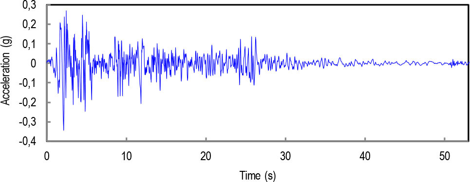
This section aims to demonstrate the influence, importance, and position of control on the structure, taking into account the effect of SSI by comparing it with the case of embedding. For this purpose and for numerical application, the dynamic loading used for exciting structures (buildings) is the 1940 El Centro earthquake with North-South components (Fig. 5.)

Fig. 5.

El-centro 1940 of the N-S Components

The structure used for numerical applications is a three-story structure, and the data is as follows:

Fig. 6.

The data of the studied model

The obtained result for the stiffness matrix of the studied soil

The Table 1 presents the natural frequencies of the first three modes for both cases, with and without SSI. It is noteworthy that the natural frequencies in the fixed case are higher than those in the SSI case.

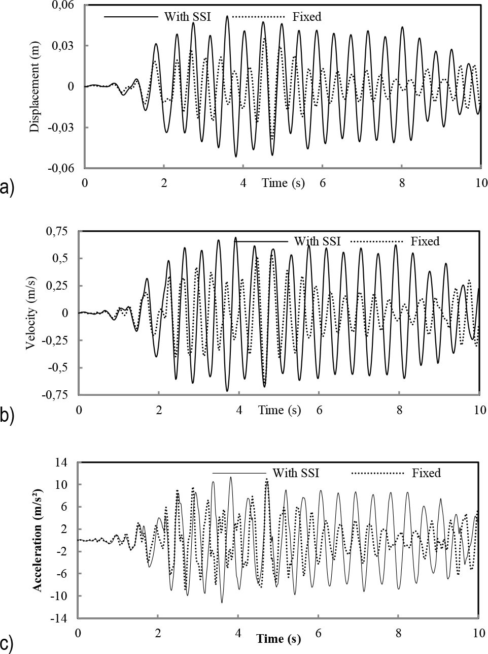
The following figure provides the displacement, velocity and acceleration history of the last floor of the model with SSI, which is compared to that of the fixed case.

Fig. 7.

The displacement, b) the velocity, and c) the acceleration of the final floor of the studied model, considering the effect of SSI, compared with the fixed case without control

Now, let's assume that the model is controlled by an active tendon system placed on the first floor for the case with ISS, and on the last floor for the case without ISS. The algorithm used is the GOAC algorithm. We will employ various values of the S/R ratios to determine the optimal S/R ratio. The results are plotted in the following figure.

Fig. 8.

Variation of maximum displacement at the last floor and maximum control force as a function of S/R ratios

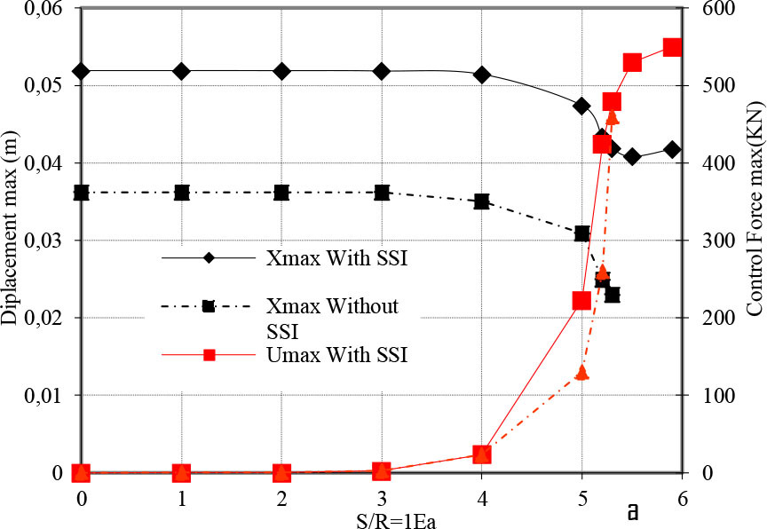
According to Fig. 8, the chosen value is S/R=2E5 for the case with ISS, and S/R=2.7E5 for the case without SSI.

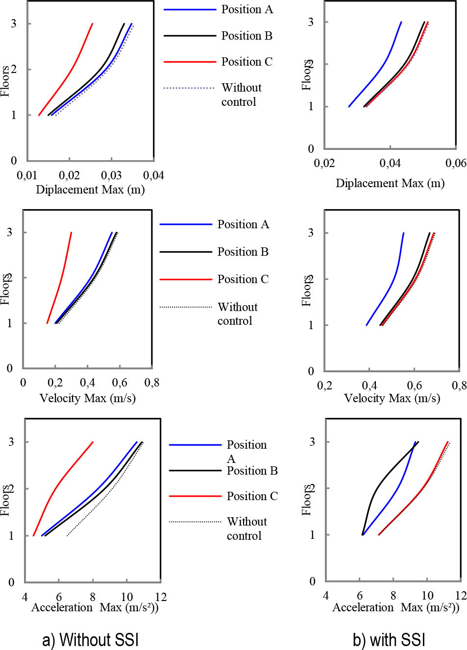
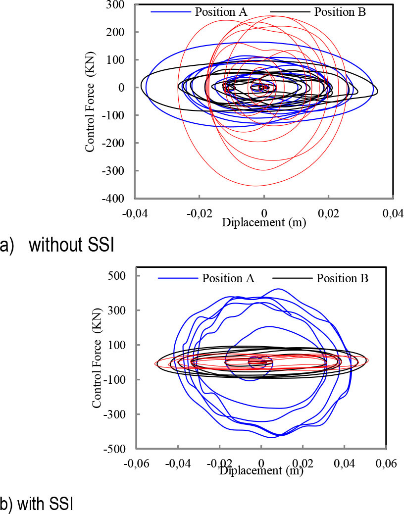
According to Fig. 9, we observe that the displacement decreases in the presence of control for both cases, with and without SSI. Additionally, the controller position has an influence on the control effect. In this model, the optimal positions are at the last floor for the case without SSI, and at the first floor for the case with SSI.

Fig. 9.

Maximum displacements, velocities, and accelerations a) without and b) with ISS for the three controller positions compared to the case without control

Fig. 10.

The control force-displacement relationship at the last floor of the studied model a) without SSI and b) with SSI for the three controller positions compared to the case without control

6. CONCLUSION

In civil engineering, modern structures are becoming increasingly complex, necessitating advanced techniques for understanding and controlling their behavior. When subjected to dynamic loads such as earthquakes or strong winds, these structures can experience significant vibrations, often leading to their failure. Despite numerous efforts to design structures capable of with-standing such loads, as evidenced by the many codes developed in this field, these structures remain highly vulnerable, with limited capacity to resist and dissipate energy. This behavior becomes even more intricate when considering that structures are founded on soils through which applied loads are transmitted, taking into account the operation of the entire soil-structure system. This phenomenon is referred to as Soil-Structure Interaction (SSI).

The most noteworthy conclusions drawn from the findings are as follows :

Overall, the study underscores the critical importance of active control strategies in mitigating dynamic responses of complex structures. Additionally, it highlights the need for careful consideration of Soil-Structure Interaction effects and optimal positioning of control elements for effective structural performance.