INTRODUCTION
Allowable heating and cooling rates for thick-walled boiler
pressure parts, together with environmental emission constraints at
different boiler loads for a
Skjervold and Nord [3] proposed a steam accumulator for a 598 MW unit with post-combustion CO2 capture as a means of improving operating flexibility. In a related study, Skjervold et al. [4] examined control concepts for adsorption-based CO2 capture under varying boiler load. Pressurised hot-water storage tanks and steam accumulators as flexibility-enhancing devices for thermal power plants were analysed by Trojan et al. [5] and Stevanovic et al. [6]. These studies show that a reliable assessment of thermal stresses in critical pressure parts is a prerequisite for flexible, safe plant operation. Stress information is also required when the temperature history of the working fluid is optimised during heating or cooling, because the permissible rate of change must be selected so that the allowable stress is not exceeded.
In horizontal pressure parts of conventional power units [7-9], and also in nuclear installations [10], start-ups and shutdowns may generate severe thermal stresses because water and steam can coexist in the same cross-section. Condensate occupies the lower portion of the element, while steam, frequently superheated, flows above it. The wall is therefore exposed to highly non-uniform circumferential heating, since the heat transfer coefficients in the water and steam regions differ markedly. In conventional plants, boiler drums, superheater inlet and outlet headers, and steam-cooler headers are particularly vulnerable to such loads. In pressurised-water reactors, comparable circumferential temperature gradients may occur near horizontal reactor inlet nozzles. Boiler codes [11] usually neglect this circumferential asymmetry and treat the wall temperature field as axisymmetric. Thermal-stress calculations in conventional and nuclear pressure components commonly assume known values of the heat transfer coefficient and fluid temperature [12]. However, both quantities are difficult to measure accurately in high-pressure, high-velocity, high-temperature flows, where dynamic temperature-measurement errors can be substantial [8].
The present work formulates a procedure for reconstructing the temperature field in an externally insulated horizontal pressure element. The input consists of wall-temperature histories measured around the circumference at a small distance from the inner surface. From these data, the transient temperature distribution in the complete cross-section is obtained. When the internal fluid temperature is also available, the circumferential distribution of the heat transfer coefficient on the inner surface can be evaluated. This coefficient is then used as a boundary condition in finite element calculations of thermal stresses in the pressure element.
MATHEMATICAL FORMULATION OF THE DIRECT PROBLEM
The transient temperature field in the horizontal pressure element is governed by the heat conduction equation:

boundary conditions:



and initial condition:

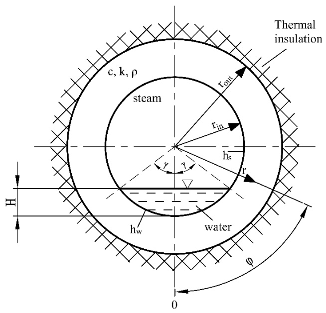
Fig. 1. Cross-section of a horizontal cylindrical header; steam flows through the upper part of the header, and condensate collects in the lower part
During heating, saturated dry steam enters the header. Initially, the internal wall surface is much colder than the incoming steam, so condensation occurs and liquid collects in the lower part of the horizontal header. The maximum condensate height is denoted by H (Fig. 1). The heat transfer coefficient in the steam region, hs, is much larger than the coefficient in the water region, hw. In the direct heat conduction problem, the inner-surface boundary conditions (1)-(3), the outer-surface boundary condition (4), and the initial condition (5) are prescribed. The resulting initial-boundary-value problem (1)-(5) is solved with the finite volume method (FVM) [13]. Figure 2 shows the discretisation of half of the header cross-section into control volumes. The circumferential direction is represented by N uniformly spaced nodes, whereas the radial direction is represented by M nodes; hence the transient wall temperature is calculated at M x N nodal points.
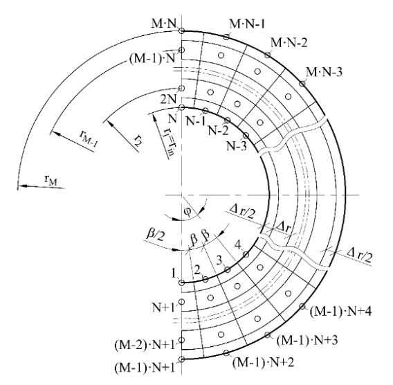
For each control volume, a heat-balance equation is written to obtain the transient temperature at each node. Representative balances are given below for a node on the internal surface, a node within the wall, and a node on the external surface. For the i-th node on the inner surface of the header (Fig. 3), the balance takes the following form:
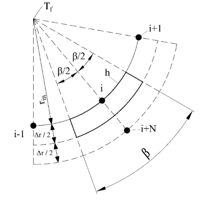
Fig. 3. Diagram illustrating the heat balance equation for the i-th node on the inner surface of the header
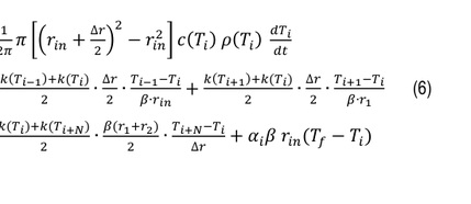
Equation (6) can be written in the following form:
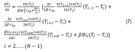
where the symbol
The balance for node (j-1)N+i, located inside the wall, is derived next (Fig. 4).
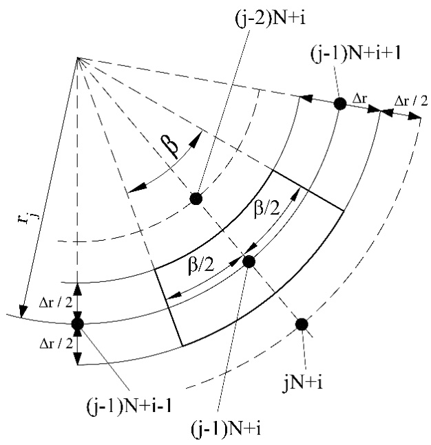
Fig. 4. Diagram illustrating the heat balance equation for node (j-1)N+I, i=2. … .(N-1) ; j=2. … .(M-1) located inside the header wall
For an internal node, with i = 2, … , N-1 and j = 2, … , M-1, the heat-balance equation is:
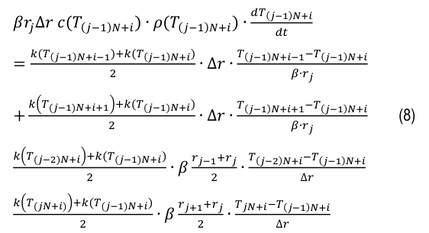
Equation (8) can be written in the following form:
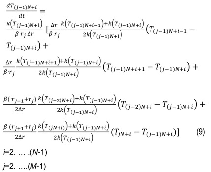
Figure 5 defines the numbering used when writing the heat-balance equation for the thermally insulated external surface of the header.
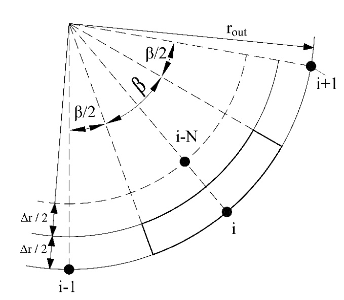
For the outer-surface nodes numbered from i = [(M-1)N+2] to i = (M x N - 1), the heat balance shown in Fig. 5 is written as:
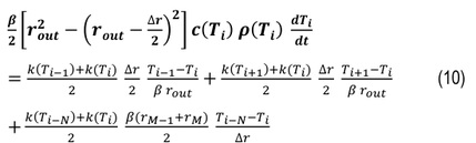
After rearrangement, equation (10) becomes:
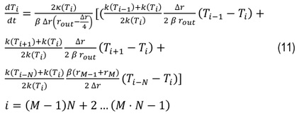
A system of (M∙N) first-order differential
equations was solved using the fourth-order Runge-Kutta method. The
solutions to the system of equations are the temperatures of the
header wall at the nodes. Changes in the internal surface temperature
around the header circumference are determined based on the
circumferential temperature distribution measured at a distance
∆r from the internal surface. By determining the
temperature distribution in the immediate area: (rin
- ∆r) ≤ r
≤(rout - ∆r), 0
≤φ ≤ π, the circumferential temperature distribution
and heat flux at the radius r = rin + ∆r
can be determined. Then, the inverse heat conduction problems in the
area rin ≤ r ≤ (rin + ∆r), 0 ≤ φ ≤ π are solved.
The solution to the inverse problem yields the circumferential
distribution of the internal header surface temperature:
T(
Tab. 1.
Thermal conductivity coefficient and thermal diffusivity of P91 steel as a function of temperature [14]
| Temperature, oC | 20 | 100 | 200 | 300 | 400 | 500 | 600 |
|---|---|---|---|---|---|---|---|
| Thermal conductivity coefficient k, W/(m∙K) | 28.7 | 29 | 29.6 | 29.7 | 29.7 | 29.6 | 29.3 |
| Thermal diffusivity, | 8.27 | 7.70 | 7.30 | 6.78 | 6.18 | 5.43 | 4.70 |
The direct and inverse calculations are presented for a header made of P91 ferritic-martensitic steel. The temperature-dependent thermal conductivity and diffusivity of this material are listed in Table 1. The inner radius is 0.1275 m, and the wall thickness is 0.05 m. The angle gamma in Fig. 1 is 37.5 degrees; therefore, the heat transfer coefficient was set to 1000 W/(m² K) at nodes 1-3 and to 3000 W/(m² K) in the steam space. The higher coefficient in the steam region reflects condensation of saturated steam on a wall whose temperature is initially lower than the steam temperature. The transient calculations assume an initial wall temperature of 20 degrees Celsius and a steam temperature of 100 degrees Celsius. The mesh contains N = 13 nodes in the circumferential direction and M = 11 nodes in the radial direction. A time step of ∆t = 1 s was used in the fourth-order Runge-Kutta integration.
MATHEMATICAL FORMULATION OF THE INVERSE PROBLEM
In the inverse problem, we know the temperature measurements at
nodes numbered from N+1 to 2N.
Considering that the outer surface of the header is thermally
insulated, the temperature in the area
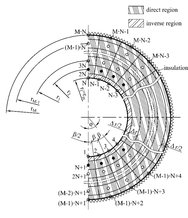
Fig. 6. Division of half of the cross-section of a cylindrical
element into finite volumes in the inverse problem; nodes located on
the radius
The heat-balance equations written for nodes N+1 to 2N are used to evaluate the temperatures at the inner-surface nodes 1 to N.
– heat-balance equation for node N+1
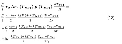
– equation (12) is used to determine the temperature
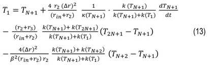
– heat balance equations for nodes
(N+i. i=2. ….
2N-1) located at a distance
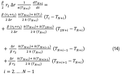
– solving equation (14) provides the expression used to calculate the temperatures of the internal-surface nodes numbered from 2 to N-1.
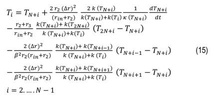
– heat balance equation for node 2N
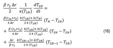
– by solving equation (16) for
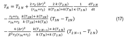
If the time variation of the fluid temperature
The HTC

where:
The heat flux

The derivative with respect to the radius in formula (19) for
COMPUTATION RESULTS
This section presents the numerical results for the direct and inverse heat conduction analyses.
Tmperature field in the horizontal-header cross-section – direct heat conduction problem
The following subsection discusses the transient temperature field obtained for the horizontal header, given the boundary and initial conditions. These direct-problem input data were specified at the end of Section 2. Figures 7 and 8 show the transient temperature distributions on the internal and external header surfaces at selected times.
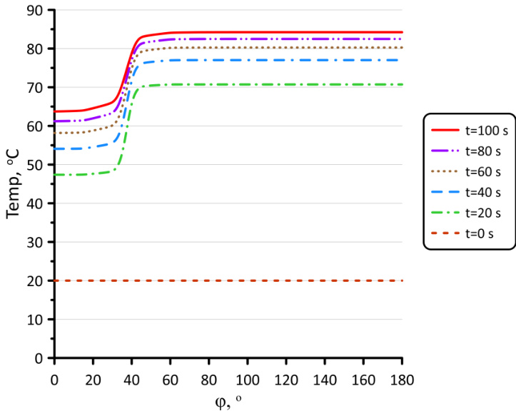
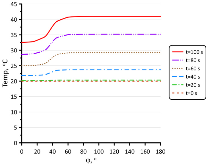
The analysis of the results presented in Figures 7 and 8 shows that
the temperature of the inner surface of the header rises faster than
the temperature of the outer surface. The temperature difference
across half the header circumference is significantly greater on the
inner surface than on the outer surface. The temperature differences
around the header circumference are caused by different HTC in the
areas where condensate and steam are present simultaneously. The
radial temperature distribution for angles
Figures 9 and 10 show that the lower part of the header warms up more slowly because the water-containing region has the lower HTC. The FVM temperatures obtained in this work were compared with results generated in Ansys. The three-dimensional temperature and stress analyses were carried out for a sufficiently long header segment so that the ends did not influence the stress state at mid-length. The model allowed free elongation and bending of the header. Several finite-element discretisations were analysed to verify mesh independence.
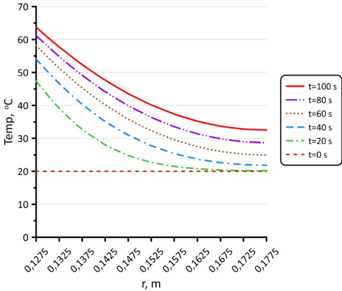
Fig. 9. Radial temperature distribution in the header wall for
selected time points
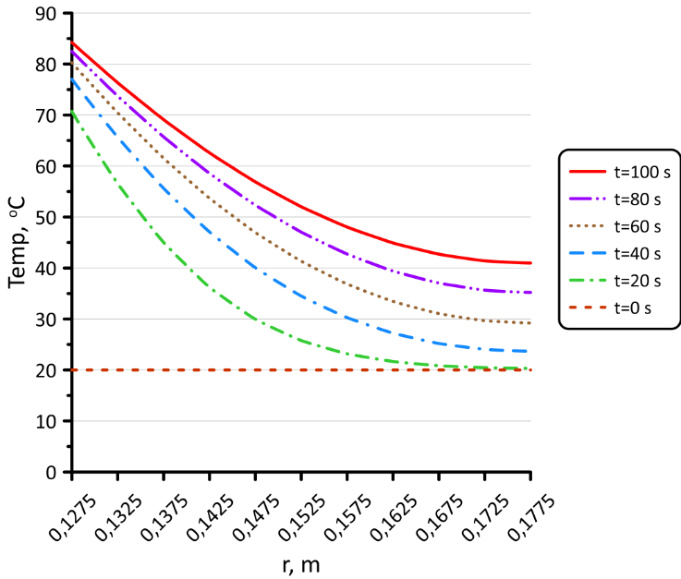
Fig. 10. Radial temperature distribution in the header wall for
selected time moments.
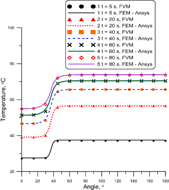
The FVM temperature histories calculated 5 mm from the inner surface were used as artificial measurement data. Figure 11 indicates very good agreement between the wall temperatures ob-tained by FVM and by FEM in Ansys.
Evaluation of the inverse-problem results
The inverse solution was used to reconstruct the header's inner-surface temperature. Temperatures at nodes N+1 to 2N, calculated by FVM and shown in Fig. 11, served as inverse-problem input data. Temperatures at nodes 2N+1 to 3N were also obtained from the FVM direct solution and are shown in Fig. 12.
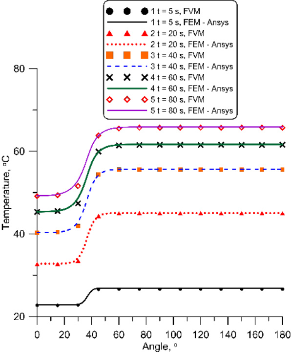
Fig. 12. Temperature of the header wall at a distance of 10 mm from the inner surface obtained from the solution of the direct problem using FVM and FEM, calculated by Ansys
Figure 12 confirms that the FVM and FEM temperature predictions are nearly the same.
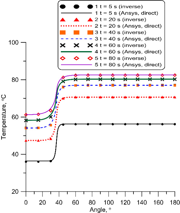
Fig. 13. Comparison of the internal header surface temperature determined from the inverse problem solution with input data determined using FEM
The inner-surface temperature obtained from the inverse heat conduction analysis was compared with the temperature calculated in Ansys (Fig. 13). The agreement is very close. Figure 14 compares the heat transfer coefficients recovered by the proposed inverse procedure with the input values used in the direct calculation. For the third-kind boundary condition imposed on the inner surface, the HTC was set to 1000 W/(m2 K) for the angular interval from 0 degrees to 37.5 degrees and to 3000 W/(m2 K) for the interval from 37.5 degrees to 180 degrees.
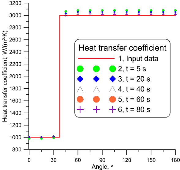
Fig. 14. Changes in the HTC on half of the inner surface of the header; 1 specified (exact) changes in the HTC; 2, 3, 4, 5, and 6 – changes in the HTC determined from the inverse problem solution for times 5, 20, 40, 60, and 80 seconds, respectively
To quantify the accuracy of the reconstructed inner-surface HTC, relative differences between the values obtained from the inverse heat conduction solution and the prescribed input data were calculated as follows:

Tab. 2.
Comparison of the HTC on the inner surface of the header determined from the inverse heat conduction problem with HTC values adopted for solving the direct problem (input data)
The results of the relative differences
Thermal stress analysis
The temperature distributions obtained in the direct and inverse regions were used to calculate the stress field in the header cross-section. The header ends were assumed to be free to elongate and bend. Temperature and stress results are presented in a section located 4 m from the free end. Additional tests were performed to evaluate the influence of FEM mesh density on the results.
Three meshes with different radial, circumferential, and axial resolutions were considered. The calculations used the following finite-element meshes:
– Mesh number 1 - 5 x 45 x 50
– Mesh number 2 - 10 x 90 x 100
– Mesh number 3 - 20 x 180 x 200
The first number in the grid designation indicates the number of
elements in the radial direction. The second number indicates the
number of elements in the circumferential direction on half of the
circumference, and the third number indicates the number of elements
in the axial direction. A comparison of the temperatures calculated at
point (rin. 0) at the bottom of the header and at point
(rin.
Tab. 3.
Comparison of temperatures in °C at point (r=rin. φ=0 ) and at point (r=rin. φ = π ). It was assumed that for an angle of 0° ≤ φ ≤ 37.5° , the HTC is 1000 W/(m2 K), while for an angle of 37.5°≤ φ ≤ 142.5°, HTC is 3000 W/(m2 K)
The analysis of the results presented in Table 3 shows that the
calculations for mesh no. 2 achieve satisfactory accuracy. Radial,
circumferential, and longitudinal stresses were determined using the
finite element mesh no. 2. Fig. 15 shows the time-dependent
temperature differences on the inner surface between
angle
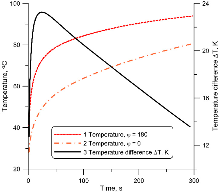
Fig. 15. The temperature difference
The top-to-bottom inner-surface temperature difference was evaluated as:

The temperature difference between the upper and lower regions results from the different HTCs. The upper region, swept by condensing steam, becomes hotter and is associated here with an HTC of 3000 W/(m² K). The lower region heats more slowly because its HTC is 1000 W/(m² K). The temperature difference ∆T reaches a maximum of 23.26 K at t = 25 s. After this peak, ∆T decreases as the header approaches thermal equilibrium.
Representative temperature and stress distributions at t = 20 s are shown in Figs. 16(a)-16(d).
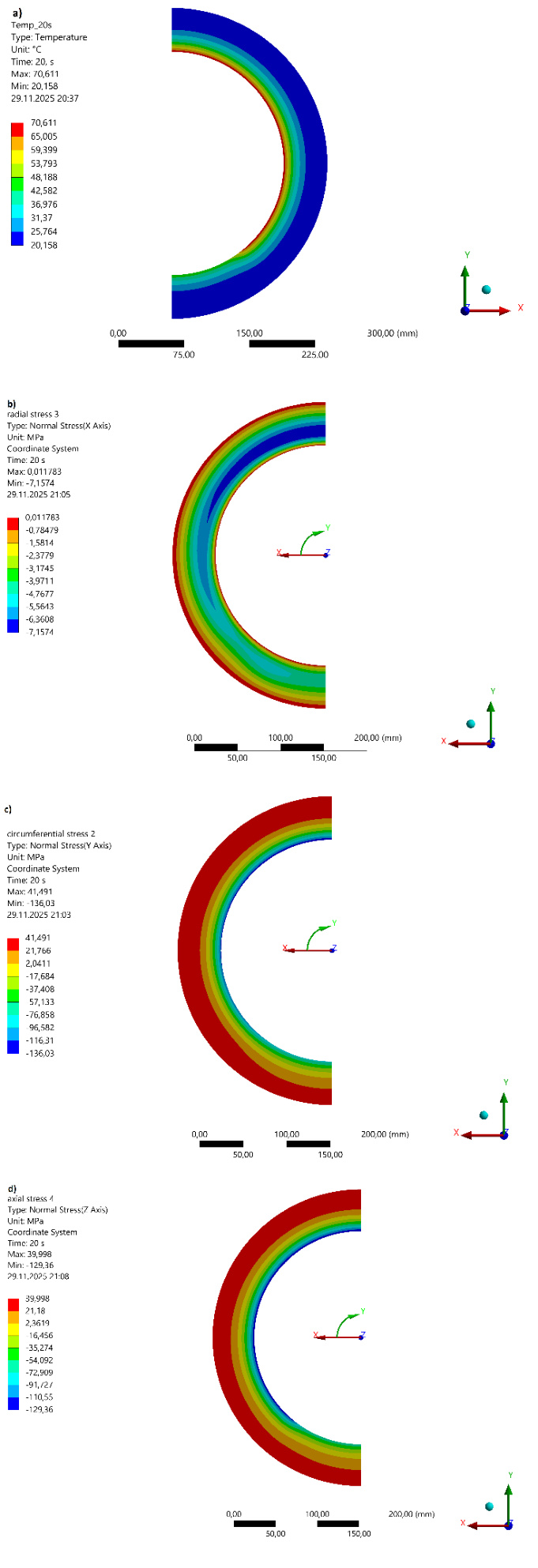
Fig. 16. Temperature and stress distribution in the middle of the header cross-section: a) temperature, b) radial stresses, c) circumferential stresses, d) axial stresses
The temperature field in Fig. 16(a) confirms that the upper part of the header is hotter than the lower part. The thermal stresses in the header cross-section are caused primarily by the temperature gradient through the wall thickness, with a smaller contribution from the circumferential temperature difference. Radial stresses are much lower than the circumferential and axial stresses (Fig. 16(b)). Considerably larger compressive stresses occur near the inner surface, while tensile stresses appear near the outer surface (Figs. 16(c) and 16(d)). The maximum circumferential tensile stress is 41.49 MPa, whereas the largest compressive stress magnitude is 136.03 MPa. Thus, the tensile stresses on the outer surface are roughly three times smaller in absolute value than the compressive stresses close to the inner surface. The axial-stress distribution follows the same pattern: the maximum tensile stress is 39.99 MPa, and the maximum compressive stress magnitude is 129.36 MPa.
CONCLUSIONS
This study proposes a method for monitoring temperature and stress distributions in the cross-section of a horizontal pressure header. Circumferential wall-temperature measurements taken a few millimetres below the inner surface are used to reconstruct the inner-surface temperature and heat flux. When the fluid temperature is measured, the heat transfer coefficient distribution on the internal surface can also be obtained. The method was verified numerically. First, artificial measurement data were generated by solving the transient direct heat conduction problem for a step change in fluid temperature from 20 to 100 degrees Celsius and for different inner-surface HTC values, with the outer surface treated as thermally insulated. Header temperatures 5 mm below the inner wall served as the measurement data. These data were then used to reconstruct the transient inner-surface temperature. After the complete cross-sectional temperature field had been obtained, the corresponding thermal-stress distribution was calculated. The tests show that wall-temperature measurements 5 mm from the inner surface are sufficient to reproduce the un-steady inner-wall temperature and the thermal-stress field across the whole header cross-section with very high accuracy. The proposed approach can therefore be applied for online monitoring of temperature and thermal stresses in headers. Knowledge of the time history of thermal stresses during start-up and shutdown also enables continuous assessment of fatigue-related durability loss in the pressure header.