
INTRODUCTION
In the ever-evolving realm of computer vision, accurately segmenting objects in video streams remains a pivotal challenge with profound implications across numerous domains. This task, crucial for applications spanning from video surveillance to human-machine interaction, including personal safety and industrial process monitoring, necessitates robust methodologies capable of dynamically adapting to changing environmental conditions.
Background subtraction [1, 2] has emerged as a widely recognized technique in video object segmentation, aiming to distinguish foreground objects from a dynamic background. Among these approaches, the median background model stands out for its effectiveness in adapting to dynamic scenes, capturing median pixel values to provide a stable background representation amidst variations such as lighting changes and moving shadows.
However, the effectiveness of background subtraction methods, including the median background model, is impeded by persistent challenges such as false positives and negatives. False positives occur when non-object regions are erroneously identified, while false negatives result from the failure to detect real objects, often due to complex variations in lighting or background dynamics.
To address these challenges, this article proposes an innovative post-processing scheme by combining the median background model with the gamma correction factor and the Mahalanobis distance metric. This synergistic approach aims to mitigate both false positives and negatives. Gamma correction enhances image contrast, facilitating the differentiation between foreground and background elements, while the Mahalanobis distance metric offers a robust statistical measure assessing the dissimilarity between pixels in difference images.
The primary contribution of this article lies in introducing an innovative post-processing scheme that significantly enhances the accuracy of video object segmentation. Focusing on the object segmentation process, we exploit enhanced difference images using fuzzy entropy and differential evolution. Fuzzy Entropy [3] resolves inherent uncertainty in difference frames, while Differential Evolution [4, 5] optimizes the segmentation process, enhancing the accuracy and efficiency of object delineation in the video stream. Subsequent sections will delve deeper into the methodology, experimental setup, and results, demonstrating how this post-processing scheme synergistically integrates with the median background model to establish a refined segmentation framework.
The paper is structured as follows: it begins by reviewing previous work on foreground detection, encompassing deep learning-based methods and traditional approaches. Subsequently, Section 3 elaborates on our MOD-BFDO method for foreground detection, which integrates background subtraction, fuzzy entropy thresholding, and differential evolution optimization. Experimental results and discussion are presented in Section 4, followed by concluding remarks in Section 5.
RELATED WORK
Detecting moving objects in video is a dynamic area of research, marked by notable advances in multi-level image thresholding and the integration of fuzzy entropy with metaheuristic algorithms like differential evolution, as demonstrated in works such as [6]. The choice of Differential Evolution (DE) among various metaheuristic algorithms stems from its balance between exploration and exploitation, making it particularly effective for optimization problems in image segmentation. DE has shown strong adaptability in handling continuous optimization problems, which aligns well with the complexity of multi-level thresholding in dynamic video sequences. These results have driven our exploration in the specific context of moving object detection. Localized approaches outlined in [7] have further piqued our interest in detecting objects within well-defined areas in video sequences. Meanwhile, global approaches to multi-level thresholding, as discussed in [8], offer crucial insights for improving detection across sequences. Li et al. (2023) introduced an approach based on the Improved Slime Mould Algorithm (SMA) combined with symmetric cross-entropy for multi-level thresholding, achieving greater accuracy in complex image segmentation tasks [9]. Additionally, Zhou et al. (2023) proposed a complex-valued encoding golden jackal optimization for multilevel thresholding image segmentation, further enhancing the robustness of image segmentation techniques [10].
Recent developments in fuzzy-based methods also play an essential role in this domain. For example, [11] introduces a robust approach to moving object detection by fusing Atanassov’s Intuitionistic 3D Fuzzy Histon Roughness Index and texture features, enhancing performance in diverse conditions. Similarly, [12] uses Atanassov’s intuitionistic fuzzy histon for robust detection in noisy environments. Another notable contribution is [13], which proposes a novel feature descriptor for moving object detection, showcasing improvements in robustness, particularly in complex scenes.
In addition to fuzzy-based approaches, the exploration of synergies between differential evolution, fuzzy entropy, and alternative entropy measures, as highlighted in [14], has broadened our understanding of multi-level image thresholding techniques. These advanced approaches can be categorized into two broad classes: methods based on deep learning and traditional unsupervised learning.
In the realm of deep learning, [15] presents a novel approach using deep neural networks for detecting moving objects, offering superior accuracy and generalization. Similarly, [16] highlights the potential of convolutional neural networks (CNNs) for robust moving object detection, while [17] uses generative adversarial networks (GANs) to generate improved training data for enhanced detection performance. Another contribution, [18], applies transfer learning to improve detection generalization across various scenarios.
In the domain of moving object detection, traditional unsupervised learning methods, such as background subtraction, temporal segmentation, and clustering, have proven effective due to their simplicity and low computational requirements. Techniques like adaptive thresholding using wavelet transforms and principal component analysis (PCA) capture spatial and temporal features, making them reliable in dynamic environments. For example, [19] introduces a method using stationary wavelet transforms for background subtraction, showing high accuracy. Similarly, [20] demonstrates temporal segmentation’s effectiveness, while [21] emphasizes the robustness of traditional approaches in specific conditions. These methods underscore the resilience and adaptability of unsupervised learning, maintaining relevance despite the rise of deep learning. Additionally, [22] explores unsupervised clustering to group objects based on temporal similarities, and [23] highlights the application of PCA for detecting moving objects in complex sequences. Traditional methods, despite their limitations, continue to be valuable in scenarios where deep learning models may be less practical due to computational or data constraints.
By consolidating these related works, our paper offers an integrated methodology for detecting moving objects in videos, emphasizing the synergies between fuzzy entropy, differential evolution, and multi-level image thresholding.
METHODOLOGY
This study focuses on improving object segmentation in video streams by combining the median background model, an innovative post-processing scheme, and advanced segmentation techniques based on entropy and differential evolution. The main goal is to achieve accurate segmentation of moving objects while overcoming the challenges of false positives and false negatives in the object delineation process.
. Calculation of Difference Images Using Median Background Model
Calculating image difference using the Median Background Model is a fundamental step in our methodology. This phase involves capturing the dynamic changes in a video sequence by subtracting the median background from each frame. The Median Background Model is presented as a robust representation of the static scene, adapting to variations in lighting, shadows, and gradual environmental changes
. Background Model Initialization
This step begins by initializing the median background model using a set of consecutive frames from the video sequence. Median pixel values are calculated independently for each pixel position on this set, creating a stable background representation.
In this context, Bkg(x, y) represents the pixel intensity of the background model at coordinates (x, y), while I(x, y) denotes the pixel intensity at (x, y) within the frame. The background model is constructed using N frames, where N signifies the number of frames incorporated within the process.
. Frame-wise Subtraction
For each subsequent frame in the video sequence, we mainly perform a per-pixel subtraction of the average background calculated from the current frame. The result is a different image that highlights the dynamic elements of the scene that stand out from the static background.
When detecting moving objects, updating the background is a crucial step. With each iteration of the algorithm, the background model is dynamically adjusted. This adaptation concerns each pixel of the matrix, and each pixel is modified according to the dynamic matrix resulting from the subtraction between the current image and the initial background. For maintaining an accurate and up-to-date representation of the background, it is essential to adopt an adaptive method. This approach takes into consideration changes observed in the scene over time. More precisely, it adjusts the values of the dynamic matrix according to new information coming from the current image. Thus, updating the dynamic matrix not only makes it possible to detect moving objects. Nonetheless, to intelligently adapt to variations in the scene to ensure robust and precise detection.
When looking closely at the difference images, it becomes apparent that some background pixels may be misclassified, thereby leading to inaccurate segmentation of foreground objects. This imprecision can compromise the overall quality of the segmentation and introduce false positive regions. It is imperative to undertake additional processing on the different images to rectify this situation. This processing process aims to eliminate these false positive areas, thereby improving the reliability of object segmentation and obtaining more accurate results in identifying elements of interest. Adopting this approach strengthens the algorithm’s ability to correctly discern the edges and details of foreground objects, thereby contributing to more robust and reliable segmentation.
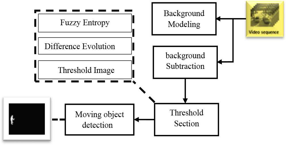
. Post-processing diagram
A new post-processing scheme is introduced to improve the results obtained by background subtraction. This system comprises two basic elements.
. Gamma correction
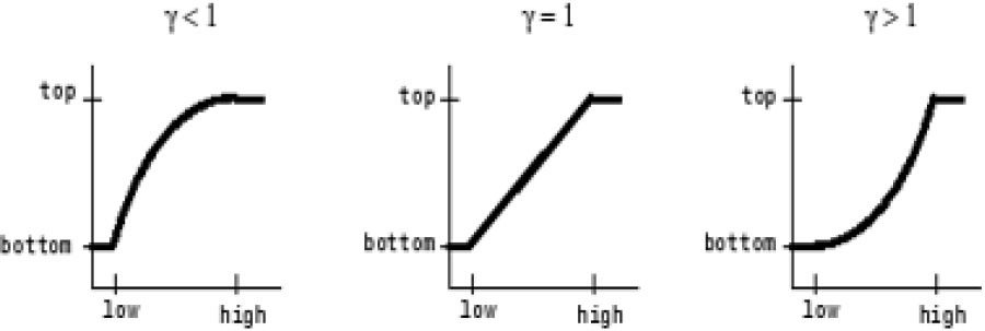
For enhancing contrast, the difference images use the gamma correction factor. By improving the ability to distinguish between foreground and background items, this improvement helps to lower the number of false positives.
Our approach consists of first defining a gamma correction factor higher than 1, which maps intensity values to lower output values, and then defining a value below 1, which extends intensity values to higher levels. Figure 3 shows the change in the output image’s intensity with the input image’s intensity values for a fixed gamma value. This lessens the low-value gris noise concentration zones.
. Mahalanobis Distance Metric
The produced different images are, then, subjected to a Mahalanobis distance calculation, which produces a refined difference image free of outlier pixels. The sample mean and covariance of the difference image—whose mean value skews toward the higher gray level values—are used in this approach. As a result, this averaging effect helps to remove ambiguity or unclearness from areas with low-valued gray levels. When it comes to reducing the impact of large covariance directions—especially those brought on by noisy components—the Mahalanobis distance is essential. Therefore, any noise is seen as an outlier and is essentially averaged out. The Mahalanobis distance metric uses the spatial orientation of the variables, taking into consideration their covariance between them.
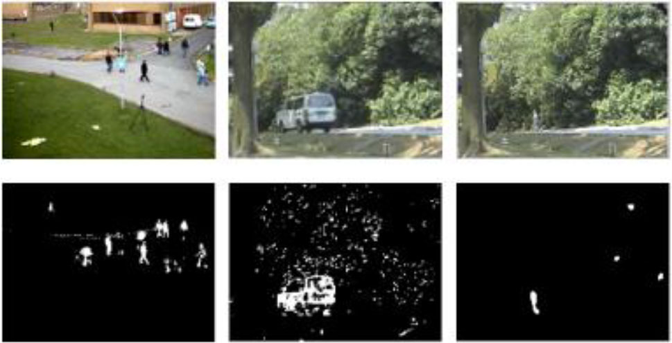
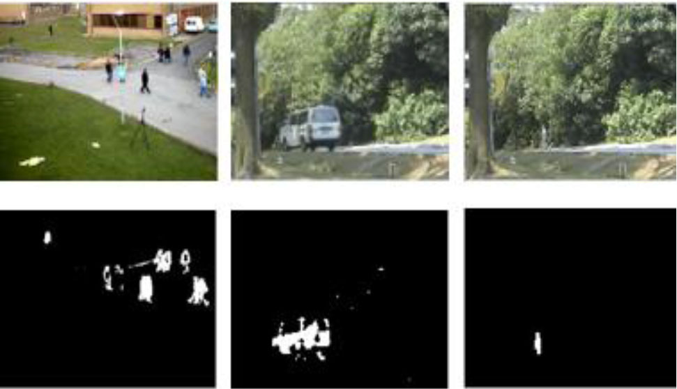
The post-processing schemes eliminated most of the gray areas present in the output. The representation of the moving object in Figure 4 is significantly more defined compared to the smudged output observed in Figure 2. The results obtained in Figure 4 also facilitate segmentation due to the elimination of several outliers.
. Object Segmentation using Fuzzy Entropy and Differential Evolution
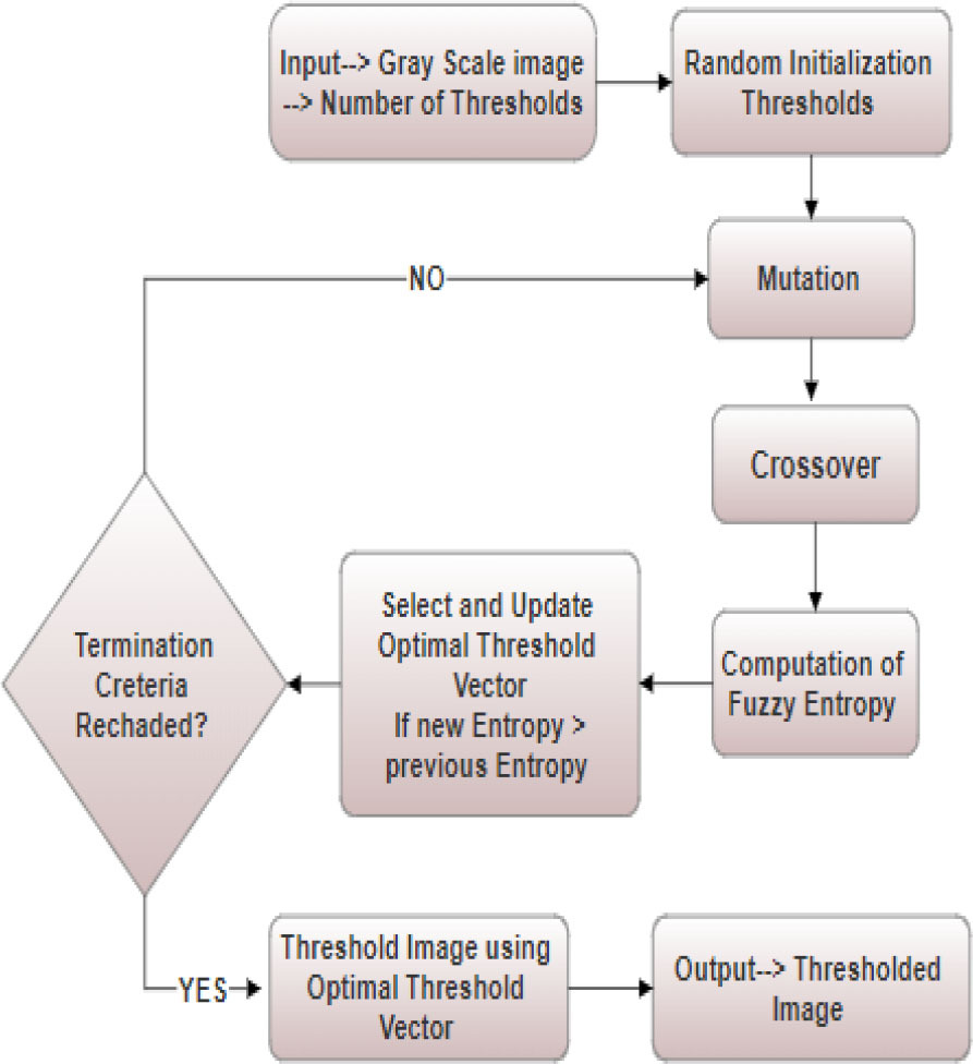
The next stage of our process is object segmentation, which is essential to fine-tuning the initial difference images. We utilize two sophisticated methods, Differential Evolution, and Fuzzy Entropy, to improve the accuracy and stability of the segmentation procedure. The local Fuzzy Entropy and Differential Evolution thresholding approach is carried out in two major stages as depicted in Fig. 5.
. Fuzzy Entropy
Fuzzy entropy is presented as a powerful tool for dealing with the uncertainty inherent in different images. In scenarios where pixel values may be fuzzy or ambiguous, fuzzy entropy captures the complexity of the pixel distribution. By incorporating the principles of fuzzy logic, it provides a nuanced measure of entropy, enabling more adaptive and accurate segmentation in regions with varying degrees of certainty.
A classical set, denoted as A, is essentially a collection of elements that may or may not be members of set A. In the realm of fuzzy sets, which is an extension of classical sets, an element can exhibit partial membership within set A. The definition of A could be stated as follows:
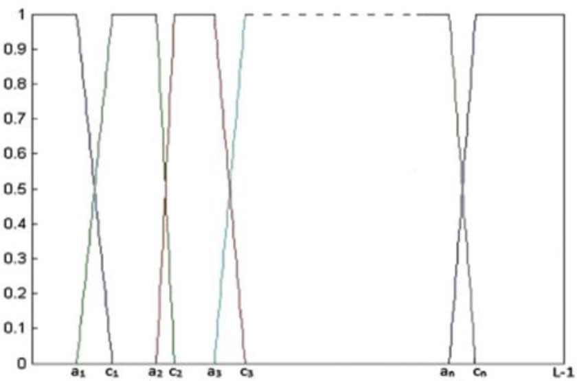
where 0 < μA(x) < 1 and μA(x) is the membership function, which measures x ‘s proximity to A.In this study, a trapezoidal membership function; as depicted in Fig. 6, is utilized to estimate the membership of n segmented areas, μ1, μ2, . . . . . , μn, by employing 2 (n− 1) unknown fuzzy parameters, namely a1, c1. . . an − 1, cn − 1, where 0 < a1 < c1 <. . . < an − 1 < cn −1 < L − 1. Then, for n-level thresholding, the following membership function can be obtained.
The maximization of fuzzy entropy at multiple levels of the image, i.e., background and foreground areas, can be formulated as follows.
(7)
Maximizing the total entropy gives the optimal value for the parameters.
It is essential to apply a global optimization technique to effectively optimize equation (8) and simultaneously reduce the time complexity of the proposed method. The (n-1) threshold values can be obtained using the fuzzy parameters as follows:
. Differential Evolution Optimization
In our approach, the optimization phase has a crucial position in perfecting the object segmentation process. To do this, we exploit differential evolution; a global optimization technique proposed by Storn [4]. This robust method adaptively adjusts the parameters of the segmentation algorithm, aiming to search for a global optimal point in a real parameter space of dimension R^D. More precisely, we use a simple version of differential evolution, called the DE/rand/1 scheme, where the ith individual of the population, represented as a vector of dimension D, contributes significantly to improving the accuracy of the segmentation process.
The first step is initialization. the set is randomly initialized in the search space, according to the following:
Where (Xjmax) and (Xjmin) define the maximum and minimum limits of the search space respectively. NP represents the total population engaged in the search process, and a rand is a random number between 0 and 1. At each iteration, for each parent, a mutant vector, called a donor vector, emerges through the differential mutation operation. Creating the ith donor vector
Where F (scalar quantity called a weighting factor) exerts its influence. The next step involves optimizing the potential diversity of donor vectors to create test vectors. A binomial crossing operation is methodically applied to each of the D variables of a vector, following a rigorous protocol.
Each j, from 0 to D, and randj in the interval [0,1], represents the jth evaluation of a uniform random generator. The component of
The previous steps are iterated until the termination criterion is met, which is defined by the number of iterations.
EXPERIMENT RESULTS
In this section, we demonstrate the intrinsic relevance of our advanced methodology through a detailed presentation of experimental results. A comprehensive comparison was made between the performance of our approach (MOD-BFDO) and other methods, including five background subtraction-based approaches: the SuBSENSE [24] approach, the SC_SOBS [25] approach, the GMM_Zivkovic [26] approach, the GMM [31] approach, and the Cuevas [32] approach, as well as a deep learning-based approach, namely DeepBS [27]. All evaluations were conducted on three distinct datasets: the SBI [29], CDnet 2014 [28], LASIESTA [30], BMC2012 [33] databases. These datasets consist of sequences captured by cameras deployed in both public and private environments, containing various moving or stationary entities within the scene, such as vehicles, individuals, and others.
. Qualitative Measurement
. Qualitative evaluation using the CDnet 2014 and SBI datasets
During this step, we proceed to analyze and evaluate the detection results obtained using our approach, while and comparing these results with those obtained by other front-end detection methods in various contexts. Experimental scenes are classified based on different criteria, such as homogeneous illumination, light contrast, presence of shadows, range, occlusion, presence of multiple targets, weak signals, and baseline. A detailed analysis of these scenes is presented as follows.
Illumination changes
Figure 7 shows the experimental results obtained under uniform illumination. The first row presents the original image, the second row exposes the ground truth image and the seventh row reveals the result of our approach. Lines 7(3) to 7(6) show the results of the DeepBS [27], SC_SOBS [25], SuBSENSE [24], and GMM_Zivk [26] methods, respectively. For the HallAndMonitor-HM video, the presented results were obtained with optimal thresholds automatically calculated by our method based on differential evolution. For NThr=4, the optimal thresholds averaged are 63.5, 128, 190.5, and 254. This choice of NThr indicates that the algorithm has determined four thresholds to segment the image. These thresholds maximize the detection of moving objects while reducing noise and false positives, offering a good compromise between accuracy and computational complexity.
Fig. 7.
Comparative analysis of our approach with state-of-the-art methods by exploiting specific videos such as “HumanBody1-HB” and “HallAndMonitor-HM” from the SBI2015 dataset. The left-to-right layout shows results for: original, ground truth, DeepBS [27], SC_SOBS [25], SuBSENSE [24], GMM_Zivk [26}, as well as our method. The results for NThr=4 are displayed in this figure
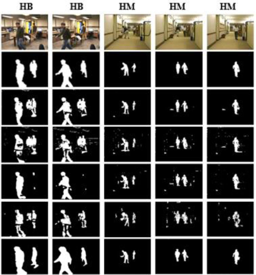
After carrying out experiments on the “HumanBody1-HB” and “HallAndMonitor-HM” videos, our approach, as well as DeepBS [27], demonstrated satisfactory performance without requiring specific quality measurements as a reference. But when it came to the detailed rendering of the target object, other leading detection methods showed less convincing results, particularly methods that tend to overlook detailed information, thus leading to detection errors.
Compared to these methods, our approach stands out for its effectiveness in eliminating slight deformations while preserving target details. This efficiency arises from the use of a multi-scale fusion model, which more adequately preserves the contours and details of the target objects.
Dynamic background
Figure 8 presents the experimental results obtained in various situations (dynamic background (CE), bad weather (SF), and shadow (BS)). The first row of Figure 8 shows the original image, the second row shows the ground truth image and the seventh row shows the result of our approach. Lines 8(3) to 8(6) correspond respectively to the results of the DeepBS [27], SC_SOBS [25], SuBSENSE [24], and GMM_Zivk [26] methods.
Fig. 8.
Comparative analysis of our approach with state-of-the-art methods by exploiting specific videos such as “SnowFall-SF”, “BusStation-BS” and “Canoe-CE” from the CDnet 2014 dataset. The left-to-right layout shows results for original, ground truth, DeepBS [27], SC_SOBS [25], SuBSENSE [24], GMM_Zivk [26], as well as our method, The results for NThr=4 are displayed in this figure
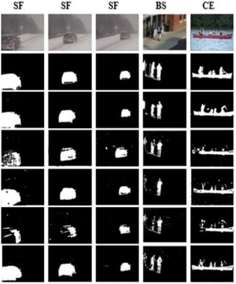
Analyzing videos with dynamic backgrounds represents a significant challenge in the field of object detection. Our approach was designed specifically to deal with this complexity, and the results obtained are very promising. Compared to several other methods, notably DeepBS [27], our approach stands out remarkably. Videos demonstrating scenes with constantly changing backgrounds are often subject to slight distortions and complex movements, making object detection difficult.
In our experiments, the results obtained by our approach and DeepBS [27] outperformed those of other methods. Figures revealing frames extracted from videos with dynamic backgrounds show exceptional clarity and accuracy in detecting target objects. Our approach, like DeepBS [27], managed to maintain satisfactory performance, even in complex conditions where other methods showed limitations.
Using Differential Evolution models in our approach has proven effective in removing slight deformations and retaining details of target objects, which is crucial in dynamic environments. These results suggest that our approach, in tandem with DeepBS [27], constitutes a particularly robust and satisfactory solution for object detection in videos with dynamic backgrounds, thus opening new perspectives for various applications, such as video surveillance and real-time computer vision.
Bad weather
The figure shows the performance of seven object detection methods on a video sequence captured under bad weather conditions. The first two rows present the original images and the ground truth, respectively. The results of the different detection methods are displayed in rows 3 to 7.
In general, deep learning-based detection methods, such as DeepBS and our approach, achieve better results compared to non-deep learning methods like GMM_Zivk [26], SuBSENSE [24], and SC_SOBS [25]. This is likely due to the ability of deep learning-based methods to learn object characteristics, allowing for more accurate identification in challenging conditions.
In this experiment, our approach determined four thresholds to segment the bad weather video, with the optimal values averaging 56.5, 107, 178.5, and 254.5. These thresholds were specifically selected to enhance the detection of moving objects while minimizing noise and false positives, ensuring a robust trade-off between detection accuracy and computational efficiency
Specifically, the DeepBS [27] method delivers the best performance on the bad weather video sequence, followed closely by our method. SuBSENSE [24] performs similarly to our method, though it is slightly less accurate than DeepBS [27]. SC_SOBS [25] produces the weakest results, though it still manages to detect some objects.
The GMM_Zivk [26] method yields the poorest performance on the bad weather video sequence, likely due to its reliance on simplifying assumptions about the object distribution. These assumptions may not hold in real-world conditions, leading to a significant loss in accuracy.
Baseline
The figure shows the results of seven object detection methods on two video sequences, one of road traffic and one of pedestrians. Rows 1 and 2 of the figures show the original images and the ground truth, respectively. Lines 3 to 7 show the results of the different detection methods.
In general, deep learning-based detection methods (DeepBS [27]) and our method achieve better results than non-deep learning-based methods SC_SOBS [25], SuBSENSE [24], and GMM_Zivk [26]. Probably, it is because our method and deep learning-based methods can learn the characteristics of the objects to be detected, which allows them to detect objects under difficult conditions accurately.
Fig. 9.
Comparative analysis of our approach with state-of-the-art methods by exploiting specific videos such as “Highway-HG” and “Pedestrians-PD” from the CDnet 2014 dataset. The left-to-right layout shows results for original, ground truth, DeepBS [27], SC_SOBS [25], SuBSENSE [24], GMM_Zivk [26], as well as our method. The results for NThr=4 are displayed in this figure
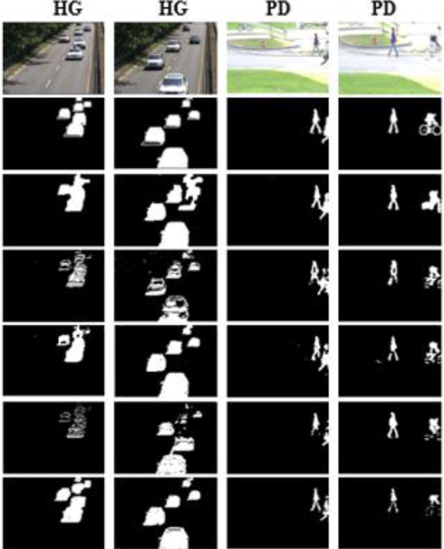
Specifically, our method obtains the best results on the road traffic sequence, followed by the DeepBS [27] method. The SuB-SENSE [24] method obtains good results on both sequences, but it is slightly less precise than DeepBS [27] and our method. The SC_SOBS [25] method obtains results comparable to those of SuBSENSE [24]. The GMM_Zivk [26] method obtains the worst results on both sequences because the GMM_Zivk [26] method relies on simplifying assumptions about the distribution of the tracked objects. These assumptions may not be valid in real-world conditions, resulting in a loss of accuracy.
. Qualitative evaluation using the LASIESTA and BMC2012 dataset
Figures 10 and 11 demonstrate the performance of the MOD-BFDO approach on two challenging sequences from the LASIESTA dataset. In Figure 10, the method handles moderate shadows effectively, accurately detecting and segmenting moving objects with minimal errors, showing robustness in controlled indoor environments. In contrast, Figure 11 highlights the method’s challenges with dynamic backgrounds, camouflage, and hard shadows, where some moving objects are not fully detected. Despite these limitations, the approach still performs reasonably well in such complex scenarios. Overall, the results indicate that the MOD-BFDO approach is effective for object detection but may struggle in environments with high background complexity.
Fig. 10.
Qualitative Performance of the MOD-BFDO Approach on I_BS_01 (Bootstrap, Moderate Shadows): (a) Original Image, (b) Grayscale Image, (c) Ground Truth, (d) Proposed Approach. The results for NThr=4 are displayed in this figure
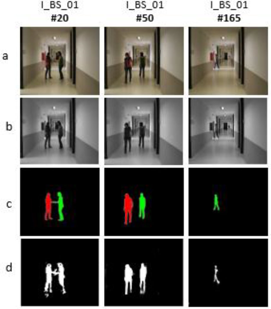
Fig. 11.
Qualitative Performance of the MOD-BFDO Approach on O_SU_01 (Dynamic background, camouflage, hard shadows.): (a) Original Image, (b) background model, (c) Ground Truth, (d) Proposed Approach. The results for NThr =4 are displayed in this figure
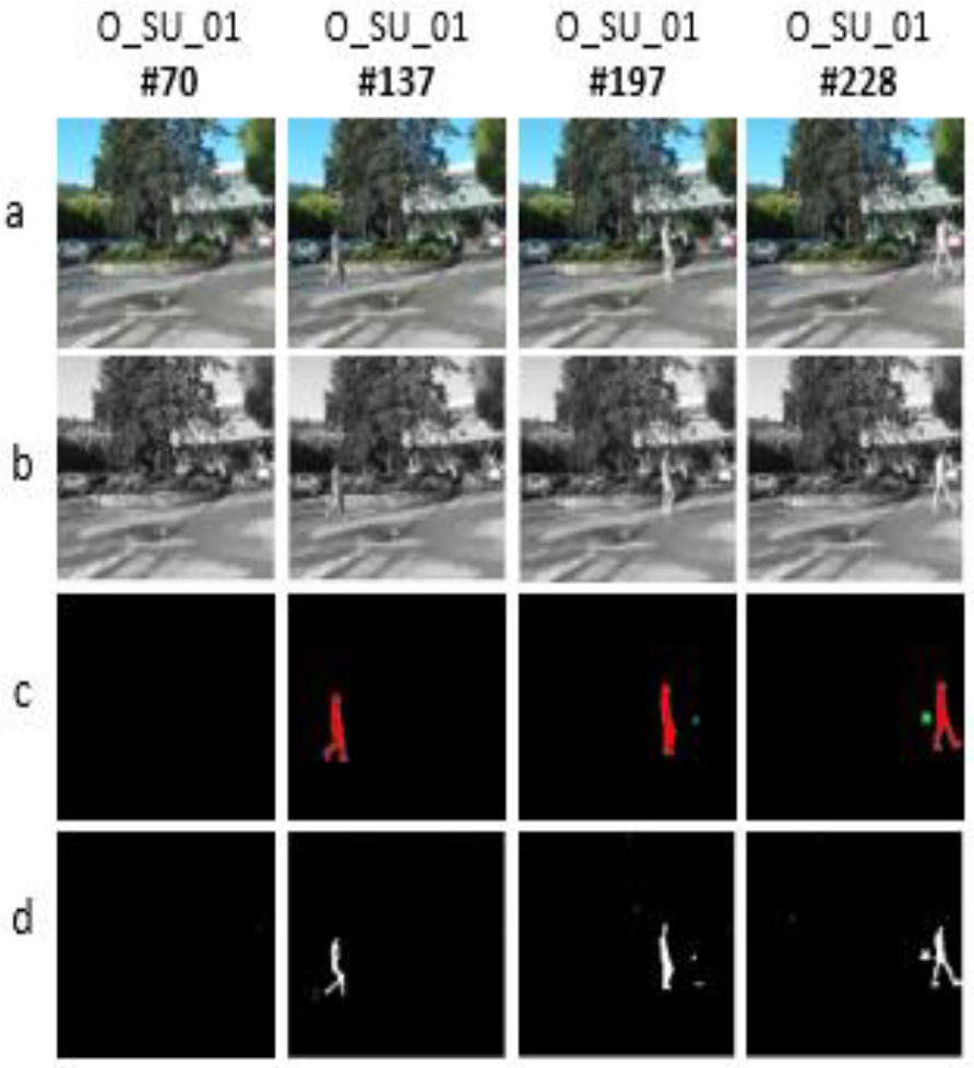
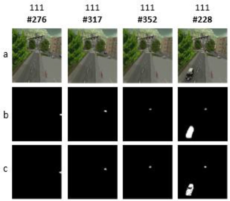
Figure 12 showcases our approach’s capability in outdoor environments, where varying lighting and small-scale movements often present challenges. The sequence images #276, #317, #352, and #228 reveal that our approach is proficient at detecting prominent moving objects even against complex urban backdrops, though smaller or distant objects may sometimes be less accurately captured, with the optimal values averaging 56.5, 107, 178.5 and 254.5.
. Quantitative Measurement
In this section, we provide a detailed quantitative evaluation of the MOD-BFDO method. The performance is assessed using various metrics that measure the accuracy and reliability of the detection results. These metrics offer a clear indication of how well the proposed approach distinguishes moving objects from the background in different scenarios. By comparing our results to existing methods, we highlight the effectiveness and robustness of MOD-BFDO in both controlled and complex environments. The following subsections provide the mathematical definitions and full forms of each metric used in our evaluation.
− RE (Recall): Measures the proportion of actual positives correctly identified.
where TP represents true positives and FN represents false negatives− SP (Specificity): Represents the proportion of actual negatives correctly identified.
where TN represents true negatives and FP represents false positives.− FPR (False Positive Rate): The proportion of false positives among all actual negatives.
− FNR (False Negative Rate): The proportion of false negatives among all actual positives.
− PWC (Percentage of Wrong Classifications): Indicates the percentage of incorrectly classified instances (false positives and false negatives) out of the total number of classifications.
− F-M (F-Measure): The harmonic mean of precision and recall, providing a balance between the two
− PR (Precision): Measures the proportion of correctly predicted positives out of all predicted positives.
. Quantitative evaluation using the CDnet 2014 dataset
Table 1 shows seven evaluation metrics for our moving object detection approach based on background subtraction, fuzzy entropy thresholding, and differential evolution optimization (MOD-BFDO) using the CDnet 2014 dataset. Our methodology has been tested in various scenarios, including uniform lighting conditions, shadow areas, long-range scene occlusion environments, the presence of multiple targets, and weak signals. MOD-BFDO effectively adapts to dynamic backgrounds and fast-moving objects, as well as slow background changes and static objects in scenes.
Tab. 1.
Evaluation of our method on the CDnet 2014
The advantages of MOD-BFDO are supported by the high precision, recall, F-measure and PWC scores shown in Table 2. Notably, MOD-BFDO shows higher recall and F-measure, as well as lower PWC, highlighting its ability to detect foreground and background pixels while minimizing errors. Compared to many traditional approaches, including those outside the deep learning domain, our method also outperforms deep learning-based models, approaching the performance of the SuBSENSE [24] algorithm in terms of accuracy.
Tab. 2.
Comparative assessment of F-measure in six categories using four methods. Each row presents results specific to each method; each column displays the average scores in each category
| Methods | F-M | ||||||
|---|---|---|---|---|---|---|---|
| Baseline | Bad weather | Dy. Backg | Shadow | Cam. Jitter | Law Fram | Overall | |
| DeepBS [27] | 0.9580 | 0.8301 | 0.8761 | 0.9304 | 0.8990 | 0.6002 | 0.8490 |
| SC_SOBS [25] | 0.9333 | 0.6620 | 0.6686 | 0.7786 | 0.7051 | 0.5463 | 0.7158 |
| SuB-SENSE[24] | 0.9503 | 0.8619 | 0.8177 | 0.8646 | 0.8152 | 0.6445 | 0.8257 |
| GMM_Zivk [26] | 0.8382 | 0.7406 | 0.6328 | 0.7322 | 0.5670 | 0.5065 | 0.6696 |
| MOD-BFDO | 0.9409 | 0.8834 | 0.9051 | 0.8785 | 0.8332 | 0.6800 | 0.8535 |
In comparison with other ranked methods on the dataset in Table 3, MOD-BFDO stands out once again, especially in terms of F-measure scores, which combine recall and precision. Even in the Law framerate category, where some approaches use more sophisticated frame-level motion analysis techniques, our method excels. Overall, we maintain the highest F-measure scores in four out of six categories, surpassing the second-best method with an 8.53% relative improvement in the overall F-measure, exclusively for the CDnet 2014 dataset. These results highlight the exceptional flexibility of our method, capable of adapting to the most challenging change detection scenarios.
Tab. 3.
A comparison between our method and some of the most important existing methods on CDnet 2014 dataset
| Methods | Overall | |||
|---|---|---|---|---|
| Avg. RE | Avg. PR | Avg. PCW | Avg. F-M | |
| DeepBS [27] | 0.8312 | 0.8712 | 0.6373 | 0. 8490 |
| SC_SOBS [25] | 0.8068 | 0.7141 | 2.1462 | 0.7158 |
| SuBSENSE [24] | 0.8615 | 0.8606 | 0.8116 | 0.8257 |
| GMM _Zivk [26] | 0.7155 | 0.6722 | 1.7052 | 0.6696 |
| MOD-BFDO | 0.8639 | 0.8492 | 0.72202 | 0.8535 |
. Statistical Stability Test
In this part, we present a comparative analysis of the performance of the MOD-BFDO method against other object detection methods, based on the mean F-measure and standard deviations calculated for each method. We then apply a z-test to assess the statistical significance of the differences between these methods.
Tab. 4.
Mean F-measure and standard deviations for different methods
| Methods | Mean F-M (µ) | Standard Deviation (σ) |
|---|---|---|
| MOD-BFDO | 0.8535 | 0.0920 |
| SuBSENSE [24] | 0.8257 | 0.1013 |
| DeepBS [27] | 0.8490 | 0.1296 |
| SC_SOBS [25] | 0.7158 | 0.1306 |
| GMM_Zivk [26] | 0.6696 | 0.1232 |
The standard deviation σ for each method is calculated using the following formula:
where:Xi
is the F-measure for each category.
̄X
is the mean F-measure for the method.
n
is the number of categories.
To compare the performance of MOD-BFDO with other methods, we use the following z-test equation:
where:̄XMOD
is the mean F-measure for MOD-BFDO.
̄Xcompared
is the mean F-measure for the compared method.
σMOD and σcompared
are the standard deviations of the respective methods
nMOD and ncompared
are the number of samples (here n=6 for each method).
The z-test was applied to assess whether the performance differences in terms of F-measure between MOD-BFDO and the other methods are statistically significant at the 95% confidence level. For this confidence level, the critical value is 1.96, meaning that any z-score greater than 1.96 or less than −1.96 indicates a significant difference.
The results show that the differences between MOD-BFDO and SuBSENSE (z = 0.498) as well as DeepBS (z = 0.069) are not significant, as the z-scores are below 1.96. However, the differences with SC_SOBS (z = 2.11) and GMM_Zivk (z = 2.93) are statistically significant, indicating that MOD-BFDO significantly outperforms these two methods at the 95% confidence level. These results confirm the robustness and effectiveness of MOD-BFDO in complex environments, particularly in comparison with older methods such as SC_SOBS and GMM_Zivk.
. Quantitative evaluation using the LASIESTA dataset
The results from both tables provide a comparative evaluation of different methods applied to the LASIESTA dataset. In Table 6, our proposed approach demonstrates strong performance, with an average F-measure of 0.8390 and high scores in categories I_SI (0.9089) and O_SU (0.8938), indicating robust capability in detecting objects in diverse environments. In comparison, Table 7 shows the results of other methods. Our method outperforms the GMM [31] and GMM_Zivkovic [26] approaches in terms of overall F-measure (0.8390 vs. 0.6880 and 0.7450, respectively) and slightly surpasses the Cuevas approach (0.8390 vs. 0.8155). This highlights the enhanced efficiency of our algorithm in handling complex and heterogeneous scenes.
Tab. 5.
Z-scores for MOD-BFDO vs other methods
| Comparison | z-Score |
|---|---|
| MOD-BFDO vs SuBSENSE | 0.498 |
| MOD-BFDO vs DeepBS | 0.069 |
| MOD-BFDO vs SC_SOBS | 2.11 |
| MOD-BFDO vs GMM_Zivk | 2.93 |
Tab. 6.
Results obtained by the proposed algorithm on the LASIESTA dataset
| Category | RE | PWC | F-M | PR |
|---|---|---|---|---|
| I_SI | 0.8969 | 0.5501 | 0.9089 | 0.9219 |
| I_CA | 0.7930 | 1.2835 | 0.8415 | 0.9250 |
| I_BS | 0.7015 | 0.4164 | 0.7120 | 0.7457 |
| O_SU | 0.8868 | 0.1917 | 0.8938 | 0.9038 |
| Average | 0.8195 | 0.6104 | 0.8390 | 0.8741 |
Tab. 7.
Comparative assessment of F-measure across four categories using four methods on the LASIESTA dataset. Each row presents the results for a specific method, while each column displays the average scores for each category
| Methods | F-M | ||||
|---|---|---|---|---|---|
| I_SI | I_CA | I_BS | O_SU | Overall | |
| GMM [31] | 0.8328 | 0.8272 | 0.36941 | 0.7240 | 0.6880 |
| GMM_ | 0.9054 | 08320 | 0.5330 | 0.7100 | 0.7450 |
| Zivk [26] | |||||
| Cuevas [32] | 0.8805 | 0.8440 | 0.6809 | 0.8568 | 0.8155 |
| Our approach | 0.9089 | 0.8415 | 0.7021 | 0.8938 | 0.8390 |
. Real-time assessment
In this section, we compare the average frames per second (FPS) across several algorithms using videos from the SBI2015, CDnet 2014 and LASIESTA datasets. To assess processing speed, we selected four videos with resolutions of (320×240, 352×288 and 720×480). All videos were recorded at 25 fps, and frames were converted to grayscale before applying the algorithms. Table V summarizes the average FPS results obtained on our system, equipped with an Intel(R) Core (TM) i7-4700MQ CPU @ 2.40GHz and implemented in C++.
For real-time applications, GMM_Zivkovic [26] emerges as the most suitable method due to its high FPS performance. MOD-BFDO offers a balanced alternative, providing a compromise between speed and accuracy. On the other hand, SC_SOBS [25] and SuBSENSE show lower FPS, especially for larger videos, which makes them less ideal for real-time scenarios involving high-resolution content.
CONCLUSION
In conclusion, our experimental results conclusively demonstrate that our MOD-BFDO method represents a significant advance in detecting moving objects in videos. Compared to object detection algorithms, whether based on deep learning or not, our approach stands out for its ability to provide superior performance, especially in difficult conditions such as lighting variations, long ranges, baseline changes, and other complex scenarios.
The innovative combination of background subtraction, fuzzy entropy-based multi-level image thresholding, and differential evolution algorithm achieved remarkable results. Background subtraction provides a crucial first step to isolating moving objects, while multi-level image thresholding based on fuzzy entropy improves robustness to environmental variations.
The optimization of the fuzzy entropy threshold parameters by the differential evolution algorithm was instrumental in obtaining superior performance. This iterative approach made it possible to maximize the detection of moving objects, while minimizing false positives, thus strengthening the precision and reliability of our method.
In summary, the results of our experiments position our MOD-BFDO method as a promising and competitive solutions for detecting moving objects. These advances open up exciting prospects for applying our method in areas such as surveillance, robotics, and computer vision, demonstrating its potential to address the complex challenges of detecting moving objects in dynamic and varied environments.