
Introduction
Pipe transportation of fluid pipeline is a critical component of the global energy supply chain. However, frictional resistance along pipe walls leads to pressure losses, reducing operational efficiency and limiting throughput capacity while increasing energy costs. To mitigate these challenges, various drag reduction techniques have been developed and studied, each offering distinct advantages and limitations [1–4]. Enhancing flow efficiency and minimizing energy consumption are key objectives in pipeline systems. Researchers have explored several approaches to drag reduction, which can be broadly categorized into three main strategies: mechanical modifications, advanced methodologies, and chemical additives.
One of the most extensively studied methods for reducing frictional losses in pipes is the use of drag-reducing additives (DRAs), such as polymers and surfactants. High-molecular-weight polymers are commonly used in pipe flows due to their ability to suppress turbulence. When introduced into a turbulent flow, these polymers elongate and align with the flow direction, damping turbulent eddies that would otherwise dissipate energy. This phenomenon, known as the Toms Effect [5–7], significantly reduces the pressure drop across the pipeline. Examples of commonly used polymers include polyacrylamide (PAM) and polyethylene oxide (PEO). In contrast, surface-active agents, or surfactants, are widely employed for drag reduction, particularly in tubes transporting Newtonian fluids such as water. Surfactants modify turbulent flow characteristics by forming micellar structures, which help suppress turbulent fluctuations and create smoother flow profiles [8, 9]. Under specific conditions, such as appropriate concentration levels (above the critical micelle concentration) and sufficient shear rates, surfactants self-assemble into elongated micelles. These micelles align with the flow direction, effectively altering turbulent energy dissipation and significantly reducing drag. Unlike polymers, surfactants exhibit a self-healing property, allowing micelles to regenerate after mechanical degradation, making them particularly suitable for long-distance pipe applications [10, 11]. Surfactants have been extensively investigated as an energy-saving solution for Newtonian turbulent flow in pipelines. Research indicates that, in some cases, they can achieve drag reduction efficiencies of up to 70%. However, their effectiveness is highly dependent on factors such as temperature, concentration, and fluid compatibility. Consequently, careful optimization of these parameters is essential for maximizing surfactant performance in pipeline systems [12, 13].
Another significant study focused on simulating turbulent flow of drag-reducing fluids in pipelines using enhanced non-Newtonian turbulence models based on the RKE and RNG formulations. A significant modeling contribution was presented by Niazi et al [14, 15]. They developed an enhanced k–ω turbulence model integrated with a modified Generalized Newtonian Fluid formulation to represent the rheological behavior of drag-reducing agents (DRAs) in turbulent pipe flows. Their study combined mathematical modeling and CFD implementation using (UDFs) to capture viscoelastic and non-Newtonian characteristics of DRA solutions [16, 17]. The model achieved strong agreement with experimental data, demonstrating improved prediction of friction factors within an average deviation of 10.5% and enhanced accuracy in near-wall regions, particularly the viscous and buffer sublayers. An experimental investigation was recently carried out using a rotating-disk apparatus to assess the drag-reduction performance of various polymer suspensions in crude oil Dastbaz [18].
Surface modification is another effective technique for reducing drag in pipe flows. This approach involves altering the chemical or physical properties of the inner tube wall surface to minimize frictional resistance. By decreasing surface roughness or enhancing the fluid's laminar characteristics near the wall, these modifications improve the interaction between the fluid and the pipe wall. One widely studied method is the application of hydrophobic or superhydrophobic coatings. These coatings repel water and other fluids, reducing adhesion and drag. Research indicates that superhydrophobic surfaces can create a thin air layer, or "plastron," on the pipe wall, acting as a slip boundary and significantly lowering frictional drag. For instance, Choi et al. [19] demonstrated that superhydrophobic surfaces can reduce drag in turbulent flow conditions by up to 30%, highlighting their potential for Newtonian fluids [19, 20].
Recent studies have also explored the effectiveness of micro-structured surface patterns, such as riblets or grooves, in reducing drag. Inspired by natural structures like shark skin, whose microscopic grooves minimize water resistance, these designs influence turbulent flow structures near the wall, thereby decreasing drag [21]. Experimental findings show that riblets can achieve drag reduction of up to 10% in turbulent channel flows. Additionally, bio-inspired convergent-divergent riblet patterns have been investigated for their ability to modify boundary layer characteristics and further enhance drag reduction [22, 23].
The application of low-surface-energy coatings, such as fluoropolymers and silicone-based compounds, has been shown to effectively reduce drag in pipe flows by minimizing fluid adhesion to pipe walls. For instance, the DragX™ surface treatment system utilizes nanocomposite technology to create a low-friction, water- and oil-repellent surface, significantly reducing surface roughness and drag resistance. Furthermore, studies have demonstrated that applying hydrophobic coatings to pressurized tubes decreases head loss, indicating reduced drag. Due to their versatility and compatibility with various fluid types, including both Newtonian and non-Newtonian fluids, these coatings are well-suited for a wide range of pipe-flow applications [24].
Another approach to drag reduction involves the strategic placement of flow-control barriers such as baffles, rings, and grids within pipes. These passive devices modify turbulence dynamics, disperse flow energy, and alter velocity profiles, ultimately reducing pressure losses. Specifically, turbulence control structures like grids and baffles disrupt cohesive turbulent eddies near pipe walls, weakening their intensity and lowering drag. Recent studies have explored the design of minimal baffles to destabilize turbulence in pipe flows, demonstrating their effectiveness in reducing frictional losses in industrial pipe systems [25]. Vortex generators (VGs) represent another type of flow barrier designed to induce controlled vortices in the fluid, promoting mixing and reducing velocity gradients near the wall. By lowering shear stress, these devices contribute to drag reduction. Zhu et al. [26] investigated the effects of passive VGs on wind turbine airfoils undergoing pitch oscillations, reporting significant aerodynamic improvements and demonstrating how VGs can effectively reduce drag in turbulent flows. These devices are particularly effective in high Reynolds number regimes. A promising drag reduction strategy involves the use of energy promoter devices strategically positioned within pipes to modify flow dynamics. Energy promoters enhance flow efficiency by reducing frictional resistance and disrupting turbulence. Their effectiveness depends on factors such as placement, height, and design. Al-Kayiem and Khan [27] have studied the influence of energy promoter height on flow structure, showing that strategically placed protrusions can alter turbulence dynamics and minimize drag. Additionally, recent research [28–31] has investigated the effectiveness of streamlined turbulence modifiers in pipe flow. These studies indicate that by dispersing energy and lowering velocity gradients near pipe walls, turbulence modifiers can significantly alter flow behavior. Experimental evaluations confirm their potential for substantial drag reduction while maintaining flow stability. These findings highlight the importance of geometric optimization and strategic positioning of turbulence modifiers in enhancing pipe-flow efficiency under turbulent flow conditions [32].
This study investigates the use of integrated energy promoters in the form of rings within circular pipes to enhance turbulent flow performance and reduce drag through computational fluid dynamics (CFD) modeling. Two geometric designs, simple and curved, were proposed to analyze how promoter shape and spacing influence flow structure, turbulence modulation, and energy dissipation. The base dimensions of both designs were kept identical to ensure fair comparison, with the curved design providing enhanced surface curvature for improved turbulence control. The novelty of this work lies in developing and numerically evaluating these optimized promoter-ring geometries as a fully passive, sustainable alternative to traditional drag-reduction methods such as chemical additives or active control devices. The results offer new insights into how geometrically induced turbulence modulation can enhance hydraulic efficiency and reduce pressure losses in industrial pipe systems, particularly those operating under turbulent Newtonian flow conditions.
Methodology And Numerical Simulation
In our research paper, the methodology relies on using energy promoters to reduce drag with a slight pressure drop in a pipe by solving the Navier-Stokes equation using ANSYS Fluent software, which falls within the fluid-structure interaction (FSI) in computational fluid dynamics (CFD).
Mathematical model
The Navier-Stokes equations for the conservation of mass, momentum, and energy were used in their instantaneous, steady-state form. In a cylindrical coordinate system (r, θ, z) shown in (Fig. 1). The governing equations for the turbulent flow of an incompressible Newtonian fluid (Fig. 2) are as follows [33, 34]. The mass conservation equation can be written as follows:

The momentum equations z-direction can be written as follows:
The momentum equations r-direction can be written as follows:
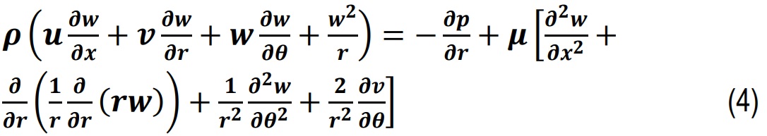
The momentum equations θ-direction can be written as follows:
In steady-state flow, the pressure distribution and velocity component remain over time, (∂)/(∂t)=0. For an incompressible fluid, the density is constant ρ=Cte, and for the axisymmetric flow, the variations in the circumferential direction are neglected, (∂)/(∂θ)=0. To ensure an accurate numerical solution, the following boundary conditions are imposed and shown in Tab. 1:
The velocity components at the pipe wall are zero in a no-slip condition:

Symmetry at the centreline: The axial velocity gradient and the radial/azimuthal velocities vanish at r=0

In the inlet and outlet of the pipe:
The velocity in the inlet and the outlet is fully developed, and the pressure is set to a reference value at the outlet.


Tab. 1
Dimensionless boundary conditions
Since the flow is turbulent (Fig. 2), a turbulence model is necessary. The Reynolds-Averaged Navier-Stokes equations with the k−ϵ model are used [35, 36]:
The Turbulent Kinetic Energy k can be written as:

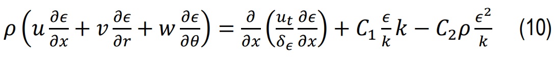
and the Turbulent Dissipation Rate ε can be written as:
In order to expand and generalize the problem, we define the non-dimensional quantities, which require the use of equations (1) to (2) and (3) in their dimensionless form:

By substituting equation (11) for the dimensionless variables into equation (1), we find:

And dividing equation (12) by U0/L, we obtain the dimensionless continuity equation:

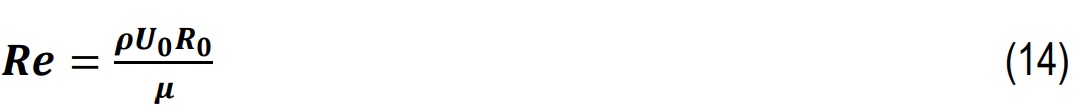
The Reynolds number (Re) can be calculated by:
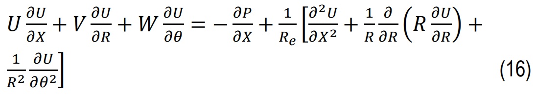
The dimensionless axial momentum equation can be written as:
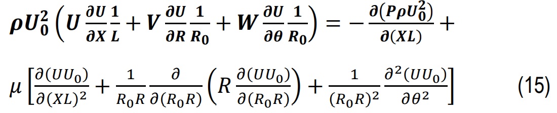
After dividing equation (15) by ρU02/L and using equation (14), it will obtain:
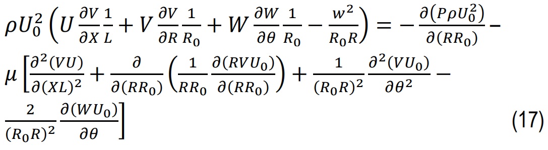
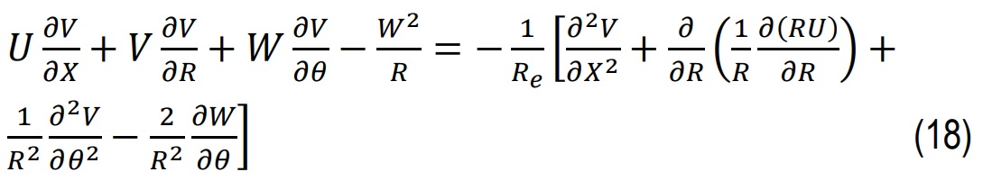
Using the same dimensionless quantities as before, Eqs. (11), (14), and substituting them into Eq. (3), it obtains the radial momentum equation as follows:
To accurately model the velocity disruptions and local shear stress induced by the energy promoters, a periodic boundary condition may be required when repeating the promoters along the pipe. This condition ensures that:
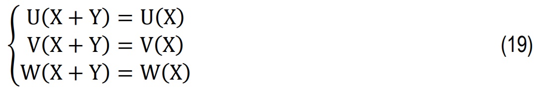
where Y is the promoter spacing and the wall shear stress τw in a pipe without the energy promoters is given by: [37]

Due to the flow disruptions and local pressure changes caused by the energy promoters, the shear stress increases in their presence. To account for this effect, a modification factor α is introduced:

where α>1 denotes an increase in shear stress brought on by the extra resistance that energy promoters create, and the value of α is influenced by the size, shape, spacing, and turbulence effects of the promoters. Where the pressure drop can be calculated by:
where feff is the modified friction factor due to energy promoters and the ϕpromoter effect can be approximated using empirical correlations based on experimental or CFD results. A general empirical form is:
CFD modelling and setup
The governing equations of ANSYS Fluent simulations were solved using the finite volume method, and the steps are shown in (Fig. 3). A Newtonian, steady-state, incompressible water flow was taken into consideration in the investigation. Grid independence research was conducted to guarantee the accuracy of the results, and a pipe segment, both with and without energy promoters, was utilized as the computational domain. The experimental setup served as the basis for defining the boundary conditions as represented in Tab. 1, which included no-slip conditions at the pipe walls, inflow velocity, and outlet pressure. The k-ε turbulence model was used to accurately estimate the effects of turbulence on drag reduction [38].

Designs of energy promoters
In order to evaluate the impact of energy promoter shape on drag reduction, two designs, one simple and the other curved, were shown in our work. These designs were chosen to investigate the effects of shape on flow behavior and turbulence modulation. Both designs' base dimensions are kept constant for uniformity in comparative analysis. While the simple energy promoter has a smooth, straightforward curve profile, the curved shape adds more surface curvature to better influence flow patterns. Fig. 4 provides a detailed illustration of these energy promoter designs together with their measurements (in millimetres) and geometric variants.
Energy promoter configuration in pipeline
A comprehensive pipe design was created to precisely assess the energy promoters' efficacy. The pipe is divided into two parts: a shorter stretch with energy promoters placed, and a longer segment without them. The region where the energy promoter rings are arranged strategically is indicated by the blue portion of the diagram in Fig. 5. Tab. 2 lists the pipeline's essential measurements.
Tab. 2
Specifications of the pipe with energy promoter
Parameter | Value (mm) |
Pipe length without an energy promoter | 29600 |
Pipe length including energy promoter | 400 |
The inner diameter of the pipe | 200 |
Pipe thickness | 10 |
Fig. 6 illustrates the placement of the energy promoter inside the pipe along the flow direction. In this study, each ring consisting of six energy promoters was designed as shown in the figure, along with the orientation of the promoters within the pipe.
Grid independence and mesh resolution
To achieve accurate numerical results, appropriate meshes for numerical simulation must be created using Ansys meshing. This is supported by Yin and Teodosiu [39], who published a study on increasing the properties of geometric meshing by improving the mesh quality at the boundary. Furthermore, certain researchers [40, 41] examined the characteristics of mesh modification concerning nodes and elements, concluding that numerical modeling is intricately linked to the mesh configuration employed, with quadratic element meshes yielding superior results compared to triangular element meshes for numerical modeling of flow through a cylinder, in both two and three dimensions [42]. This study highlights the critical relationship between mesh density and simulation accuracy.
To ensure the stability and reliability of the numerical solution, this process involves evaluating the pressure loss per unit length and analyzing the percentage error. A mesh independence study was conducted by varying the number of elements in the fluid domain within the pipe to achieve accurate and consistent simulation results. The primary metrics used to assess the impact of mesh refinement were the pressure drop per unit length and the percentage error between successive mesh refinements. The study examined element counts ranging from 2,000,000 to 12,000,000 to determine the optimal mesh density. Simulations were performed for a case with a fluid velocity of 0.5 m/s and four rings of energy promoters (EPs).
Tab. 3 illustrates the effect of mesh refinement on the accuracy of the numerical results, showing a decrease in pressure loss (ΔP/ΔL) as the number of elements increases. Initially, at lower mesh densities (500,000 to 3,000,000 elements), pressure loss decreases significantly with mesh refinement. However, beyond 7,000,000 elements, the results stabilize, indicating mesh independence and solution convergence.
Tab. 3
Data of mesh independence test
Number of Element (x 106) | ∆P/∆L (pa/m) | Percentage Error (%) |
2 | 4.55 | - |
3 | 3.817 | 16.01 |
4 | 3.385 | 11.3 |
5 | 3.157 | 6.72 |
6 | 2.991 | 5.23 |
7 | 2.903 | 2.93 |
8 | 2.835 | 2.34 |
9 | 2.773 | 2.17 |
10 | 2.744 | 1.01 |
11 | 2.717 | 0.97 |
12 | 2.693 | 0.87 |
To validate the selected mesh, the results were compared with a previous study by Al-Kayiem and Khan [27]. Fig. 7 and Fig. 8 illustrate the convergence and error percentage, respectively, demonstrating the accuracy of the obtained results. The comparison showed that the difference between the two studies did not exceed 1%, confirming the reliability of the numerical approach.
Fig. 7. Mesh-convergence results showing the variation of pressure drop per unit length (ΔP/ΔL) with increasing mesh resolution
Fig. 8. Percentage error versus mesh size between successive mesh refinements of the present study and Hussain. H’s study
Based on the convergence results, 8 million elements were found to be sufficient for conducting the simulation and obtaining accurate results. The error rate remained within 3% when compared to simulations with 9 million and 10 million elements. Each simulation took approximately 3 hours and 15 minutes, and increasing the mesh density beyond 8 million elements significantly raised computational costs. Therefore, 8 million elements were deemed optimal, ensuring accuracy without unnecessary resource expenditure.
Results And Discussions
Model validation and verification
Tab. 4 presents the comparison of pressure drop per unit length (ΔP/ΔL) between the current study and the work of Al-Kayiem and Khan across various velocities. The percentage difference between the two results is minimal, ranging from 0.05% at the lowest velocity to 0.025%, indicating a strong agreement. These slight variations confirm the accuracy and reliability of the simulation model.
Tab. 4
Pressure drop per unit length at various velocities
Fig. 10. Comparison of simulated pressure drop per unit length (ΔP/ΔL) with theoretical predictions across the tested Reynolds number range
This finding is further supported by the comparison of simulated and theoretical pressure decrease results shown in Figure 10. In this work, the classical Darcy–Weisbach equation (22) and the Colebrook equation (23) were used to calculate the pressure drop, and the effective friction factor feff taking into account the presence of energy promoters by adjusting the flow conditions [43]. The industrial pipe surface roughness, ε = 0.00015 m, was considered; the data points closely follow the trend and exhibit a linear relationship. Additionally, the error curve shown in Figure 10 shows that the percentage error sharply decreases as the Reynolds number increases. This suggests that the simulation model becomes more accurate with increasing Reynolds numbers, which further supports the reliability of the numerical predictions. The consistency between the simulation, theoretical, and error results analysis demonstrates how well the model results.
Pressure drops and variable analysis
To comprehend the effects of flow behavior and energy efficiency, a methodical examination of the major variables affecting drag reduction was carried out in this study. Among the main factors taken into account are:
Energy promoter design: Two different designs, one curved and the other simple, were examined to see how well they reduced turbulence and minimized pressure losses.
Distance between Rings: To evaluate its impact on drag reduction and overall flow performance, the distance between energy promoter rings (50 mm, 100 mm, and 200 mm) was changed.
Flow Conditions: To investigate the relationship between turbulent flow structures and energy promoter setups, simulations were run at different flow rates.
To find the best configurations, each variable was examined alone and in combination. To measure gains in drag reduction efficiency, the outcomes were compared to a baseline scenario without energy promoters. It can be seen that the pressure drop throughout the pipe at different Reynolds numbers (Re) is shown in Fig. 11 to Fig.13. Three distinct cases (1), (2), and (3) of rings with energy promoters (EPs) were spaced 200 mm, 100 mm, and 50 mm, respectively. Two EP designs, curved and simple, were examined. In each instance, the flow rate was changed while keeping six EPs in each ring. The drag reduction (DR) performance of these energy promoters was assessed in percentage terms.
The case one of 200 mm distance between rings with Reynolds numbers less than 150,000 Performance is similar for both the curved and plain designs, with just minor variations in pressure drop and with increasing Reynolds numbers, the curved design starts to exhibit a little benefit; nevertheless, if Reynolds numbers exceed 150,000: The curved design performs noticeably better than the plain design, reducing the pressure drop. This suggests that the curved promoters are better at managing turbulence and energy dissipation at greater flow rates.
However, we observe that in the second instance, the Reynolds Numbers are less than 150,000. The curved design performs marginally better than the plain design, although consistently, the curved design's streamlined structure starts to benefit from the increased flow interactions caused by the tighter spacing. Also, it can be noticed that for Reynolds Numbers greater than150,000 than the curved design's advantage becomes more pronounced, with pressure drops significantly lower than those of the simple design, and Simple energy promoters show increasing resistance, likely due to turbulence caused by their geometry.
The third case's trends show that for Reynolds Numbers less than 150,000, both designs struggle with increased flow disturbances brought on by the near spacing, but the curved promoters adapt better. The pressure declines for the two designs are quite close, but the curved design keeps a slight edge. Reynolds Numbers are greater than 150,000, although, in comparison to the simple design, which struggles with the increased turbulence at greater flow rates and results in a higher resistance, the curved design consistently reduces the pressure drop, demonstrating its superiority.
Drag reduction and velocity effect
Fig. 14 presents the velocity magnitude contours for a pipe segment in two cases: (a) with energy promoters and (b) without energy promoters. The results illustrate the effect of energy promoters on the velocity distribution, showing how they contribute to drag reduction by relieving turbulence near the wall of the pipe. This effect reduces velocity gradients and promotes a more uniform flow.
Fig. 15 illustrates the velocity magnitude contours within the pipe fitted with periodically spaced energy promoters. The results reveal distinct low-velocity regions (depicted in blue and green) forming downstream of each energy promoter, corresponding to zones of flow deceleration and localized recirculation. These recirculation regions progressively dissipate as the fluid moves downstream, allowing the velocity to recover toward its centerline value. The periodic arrangement of the energy promoters induces repetitive flow disturbances, creating alternating regions of velocity reduction and recovery along the pipe length. The velocity field is visualized using a color scale, where blue denotes low velocities and red represents the highest velocities (up to 1.25 m/s). A magnified view of a single promoter region further emphasizes the symmetrical velocity distribution and uniform spacing, confirming the effectiveness and geometric consistency of the promoter design.
Tab. 5 further confirms that both the design and spacing of energy promoters significantly influence drag reduction performance. Curved promoters consistently outperform simple ones, with the most pronounced improvements occurring at higher velocities. Closer spacing (50 mm) enhances this effect by intensifying interactions between the promoter-induced secondary flows and the main flow, leading to greater turbulence modulation and reduced frictional resistance. The maximum observed performance difference is 79%.
Fig. 16 reinforces these findings, showing that the curved 50 mm configuration achieves the highest drag reduction percentages across the entire velocity range, peaking at approximately 9%. The performance curves for all configurations exhibit a slight U-shape, with drag reduction minimizing around intermediate velocities (0.6–0.9 m/s) before increasing at higher velocities. This trend suggests that energy promoters are most effective in fully turbulent flow, where their geometric features generate strong flow separation and reattachment zones, breaking down larger vortices and effectively reducing drag.
Fig. 16. Drag-reduction percentage versus flow velocity for multiple promoter configurations and spacings
Tab. 5
Drag reduction percentage (%) for various configurations and velocity
To contextualize the obtained results, it is instructive to compare the drag-reduction efficiency of the proposed energy-promoter rings with other established methods. Riblet and micro-grooved surface designs typically achieve reductions of 5–10%, while swirl flow generators can yield 10–15%, depending on configuration and Reynolds number. Chemical drag-reducing agents such as polymers or surfactants may achieve reductions exceeding 60–70%, but their performance is often limited by shear degradation, concentration control, and high operational cost. In contrast, the promoter-ring system demonstrated a maximum drag reduction of approximately 9%, placing it within the effective range of passive flow-control strategies while maintaining structural stability, chemical-free operation, and low maintenance requirements. These characteristics highlight its potential for sustainable, long-term pipeline applications where continuous additive dosing or surface renewal is undesirable.
Flow Structure and Circulation Analysis
To further elucidate the mechanisms of drag reduction, the tangential velocity vector fields at the outlet cross-section were examined for both the smooth pipe and the pipe containing six energy promoters (Fig. 17). In the smooth pipe (a), the vectors are randomly oriented, indicating isotropic turbulence and strong circumferential mixing. In contrast, the pipe equipped with (b) exhibits organized counter-rotating secondary vortices near the wall. These coherent swirl patterns redistribute momentum from the near-wall region toward the pipe core, thereby attenuating turbulence intensity and reducing wall shear. The promoters act as flow stabilizers by suppressing chaotic tangential fluctuations and enhancing streamwise alignment of velocity vectors. This reorganization of turbulent structures explains the lower pressure-drop and friction-factor values obtained in the promoted configurations.
Conclusions And Future Works
The study's findings highlight the crucial role of energy promoter rings in reducing drag and optimizing fluid flow in turbulent Newtonian pipelines. CFD simulations in ANSYS Fluent confirm that curved energy promoters outperform simple designs, effectively reducing pressure drop and turbulence. The results indicate that drag reduction efficiency improves with decreased ring spacing, reaching a maximum reduction of approximately 9%, compared to 7% in previous studies. This comparison underscores the effectiveness of different promoter topologies and designs in mitigating pressure losses. While the curved design proves superior at higher Reynolds numbers, particularly in turbulent flow conditions, the simple design remains a cost-effective alternative for low-Reynolds-number systems, offering reasonable performance without significant efficiency losses. These findings hold valuable implications for pipeline transport systems, especially in the oil and gas industry, where reducing energy consumption and pressure losses is a major concern. While the present simulations were conducted using water as the working fluid, the physical mechanisms governing drag reduction are not fluid-specific but are instead related to flow structure dynamics. The observed attenuation of near-wall turbulence, vortex reorganization, and reduction in shear stress are expected to occur in other Newtonian liquids such as crude oil or refined fuels when flow conditions are scaled appropriately. For non-Newtonian or temperature-dependent fluids, quantitative variations in drag-reduction magnitude may arise due to rheological or thermal effects; however, the same energy-promoter geometries are anticipated to yield beneficial flow stabilization and reduced pressure losses. Future studies will extend this analysis to such fluids by incorporating viscosity-dependent and thermal-coupled models under realistic pipeline conditions. To further enhance the applicability and efficiency of energy promoters, additional research is needed. Future studies should:
Investigate the long-term impact of energy promoters on pipeline integrity and wear to ensure sustainability;
Experimentally validate CFD findings to improve the accuracy of numerical models;
Expand the analysis to non-Newtonian fluids, broadening the applicability of energy promoters for industries handling viscous and complex fluids;
Optimize ring geometry and material selection to maximize performance and explore potential efficiency improvements;
Assess the economic feasibility and cost-benefit ratio to support widespread industrial adoption.