
INTRODUCTION
In the rapidly advancing world of technology, it is essential not only to keep pace with changes but also to actively leverage cutting-edge information technologies to enhance traditional industries. This is particularly relevant to the modeling of the drying process of hygroscopic materials, such as wood, which has played a crucial role in the production of high-quality wooden products and materials for decades. This process also affects sectors such as construction, furniture manufacturing, and the packaging industry. In particular, the development of software for the computer-aided design of 3D models of drying chambers and the simulation of drying processes in them offers significant potential for increasing efficiency in these sectors.
Over the past decades, many efforts have been made to improve the design of drying chambers and increase their efficiency. Researches such as [1] and [2] emphasize the advantages of automating the design of drying chambers using modern software interfaces, in particular the SolidWorks API. In turn, research [2] focuses on the creation of simplified, operator-usable 3D models of drying chambers, while in [3], complex mathematical models developed to simulate heat and moisture exchange processes in such chambers. In addition, studies such as [4] address the problems of high-temperature drying, propose advanced mathematical approaches, including the Navier-Stokes equation, to model the related heat, and mass transfer processes.
Despite these advances, traditional modeling methods remain computationally intensive, requiring significant time and computing resources. Nevertheless, recent studies [5] and [6] show that the cellular automata method can serve as a promising alternative, offering faster modeling without compromising accuracy. For example, in [5], finite element methods are compared with cellular automata for modeling wood drying, demonstrating comparable accuracy in a two-dimensional scenario, but with reduced computational expense. Similarly, in [6], asynchronous cellular automata were successfully applied to heat conduction problems, emphasizing their potential for high-speed computing in complex systems.
Even though cellular automata demonstrate high efficiency in modeling, the possibility of integrating them with 3D models of drying chambers is still insufficiently studied. This unsolved problem emphasizes the need for further research to develop innovative solutions. These solutions can improve the efficiency and accuracy of not only the computer-aided design of 3D models of new and potentially more efficient drying chambers, but also the simulation of the drying process in them.
The object of research in this work is the process of drying hygroscopic materials in drying chambers.
The subject of the study is a cellular automata model for simulating the drying process of hygroscopic materials in drying chambers, for example wood.
The purpose of the research is the development and software implementation of a cellular automata model for simulating the drying process of hygroscopic materials, which includes a cellular automata field and corresponding rules of transitions. To achieve the set goal, the following main tasks are defined:
− Automated design of a 3D model of a drying chamber in the SolidWorks environment by using the SolidWorks API;
− Development and software implementation of algorithms for presenting this 3D model in the form of a cellular automata field;
− Analysis of mathematical models of heat and moisture transfer processes in drying chambers;
− Based on the conducted analysis, development of transition rules for the cellular automata model;
− Development of a database for saving input data, intermediate data, as well as results for each of the cells on the field;
− Modeling of drying processes of hygroscopic materials in a drying chamber by using a cellular automata model;
− Analysis and verification of obtained simulation results with real experimental data.
− The scientific novelty is as follows:
− A new model of cellular automata was developed to determine changes in the main parameters of hygroscopic material and its drying agent;
− The structure of the cellular automaton field was improved, which, in contrast to the existing ones, allows taking into account the physical and geometric characteristics of the 3D model of the drying chamber;
− algorithms for parameterization and CAD design of the 3D model of the drying chamber and its main components were developed, which makes it possible to effectively change their characteristics to specific process conditions.
The practical significance of the research is as follows:
− Saving time and material resources due to the rapid change of geometric characteristics of the 3D model of the drying chamber or its components, without the need to recreate them;
− Minimal user intervention in the process of creating a field of cellular automata with different types of cells, by developing and programmatically implementing the appropriate algorithm;
− Increasing the speed of modeling compared to the finite difference method by developing a scheme of relationships between adjacent and tangential cells and using it in conjunction with transition rules.
In this work, the 3D design method was used to create a 3D model of the drying chamber, the cellular automata method was used for modeling, and the method for determining the relative error was used to compare the simulation results.
AUTOMATED DESIGN OF THE 3D MODEL OF THE DRYING CHAMBER
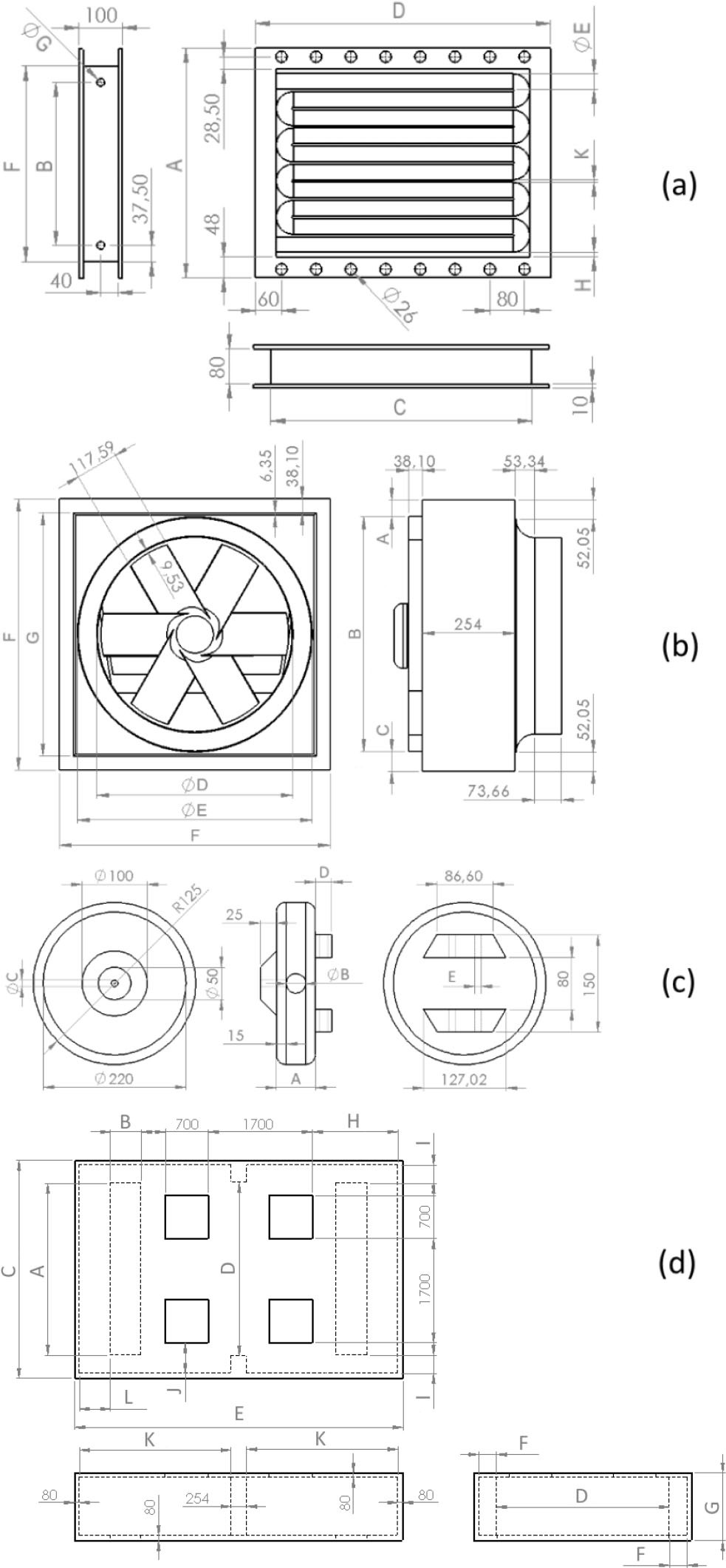
A drying chamber comprises numerous components, and designing each of them can be a time-consuming and resource-intensive task. Especially when these components are not always considered in the modeling of various physical processes, notably the drying process. To streamline the design process, it is practical to simplify by focusing on the main components, such as walls, doors, ceilings, roofs, stacks of drying material, heaters, nozzles, and fans. Each of these components serves crucial functions, including delineating the study area (doors, walls, roof, ceiling), defining the study area (stacks of drying materials), heating the drying agent (heaters), humidifying the drying agent (nozzles), and ensuring circulation of the drying agent (fans). The majority of these components can be easily coded for automated design. However, for components like material stacks, heaters, humidifying nozzles, and fans, the process becomes more intricate and involves multiple automated design steps. At each phase, relevant 2D sketches (refer to Fig. 1) are created, serving as the foundation for the development of their corresponding 3D models. Subsequently, these 3D models are amalgamated into completed assemblies, the number of which may vary depending on the design of the drying chamber and the technological process requirements [8].
Fig. 1.
View of 2D sketches of the water heater (a), axial fan (b), humidifying nozzle (c), and ceiling (d)
For the computer-aided design of the 3D model of the drying chamber, the following dimensions of the body were taken into account: height 2.25 m, width 5.703 m, length 7.291 m, with a wall thickness of 5 cm, and parameterized dimensions (refer to Tab. 1).
Tab. 1.
Parameterized dimensions of the main components of the 3D model of the drying chamber
Hence, during automated design, it is essential to utilize the primary window of the software, as depicted in Figure 2. Within this window, users can specify the nominal dimensions of the hygroscopic material, its species, and the quantity per stack. In this case, 16 stacks are designed, each containing 36 pine lumber with a thickness of 32 mm, a width of 75 mm and a length of 2.5 m. The height of the spacer between rows in the stack is automatically determined based on the height of the hygroscopic material.
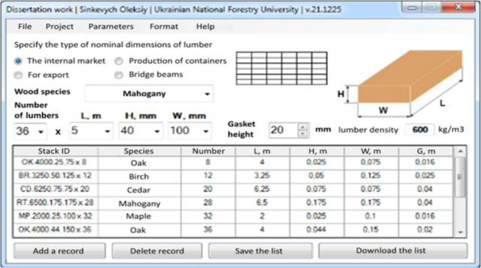
Upon selecting all the requisite parameters and clicking the “Add a record” button, a new stack identifier is appended to the database. Its ID is constructed in the following manner: the initial two letters denote the wood species code, such as “BR” for birch, “CD” for cedar, “RT” for mahogany, “MP” for maple, “OK” for oak, and so forth. The subsequent numbers correspond to the length, height, and width of an individual material, along with their quantities. This comprehensive information is crucial for the automated design of the specified stack.
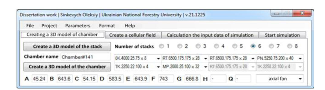
However, real drying chambers commonly incorporate multiple stacks. In light of this, the software’s first tab (refer to Fig. 3) was developed. This tab enabling users to specify the number of stacks and choose their type from the list created in the main program window (as described earlier). In essence, the user has the option to facilitate the automated design of either a 3D model of individual stacks or an entire assembly of the drying chamber. When opting for the entire assembly, it is necessary to define its name. All created 3D models are stored in the program directory by default, though users can easily customize this location in the software settings.
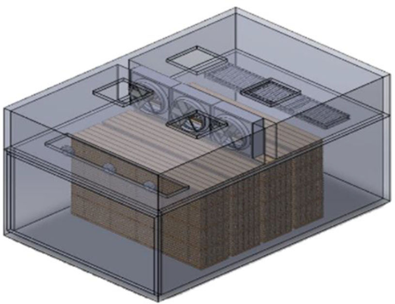
Through automated design, a 3D model of the drying chamber in SolidWorks can be obtained, as illustrated in Figure 4. The use of the SolidWorks API significantly saves time on this task.
CREATION OF A CELLULAR AUTOMATA FIELD
To create a cellular-automata field, the initial step involves creating a specific graphic scheme (refer to Fig. 5), that illustrating the systematic process of transforming the 3D model of stacks. Similarly, the process of converting the 3D model of the drying chamber will take place.
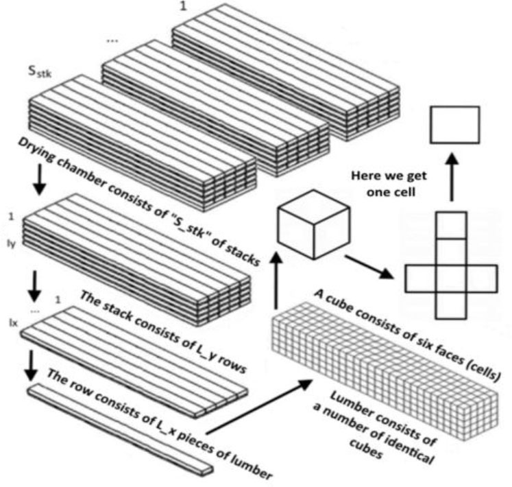
The creation of a cellular automata field [9] involves the following steps:
The program retrieves the dimensions of the dried materials in stacks, including “L” for length, “H” for height and “W” for width.
The program retrieves the maximum allowable division density of the 3D model (dm), calculated across the greatest common divisor among its dimensions.
The program retrieves the desired level of division (di), indicating the precision of the calculations. Higher levels of division result in increased time and resource expenditure.
The program determines the final division density (d), which defines the cell sizes. All cells possess identical face dimensions.
The program reads the number of drying materials in one stack (Slmb) and determines the number of materials in one row (lx) and the number of rows (ly) in one stack. Additionally, the program reads the number of stacks (Sstk).
The program retrieves the total number of cells on the cellular automata field for each of the three coordinates (Sx, Sy, Sz).
The program creates a three-dimensional array (a), where the elements represent cells.
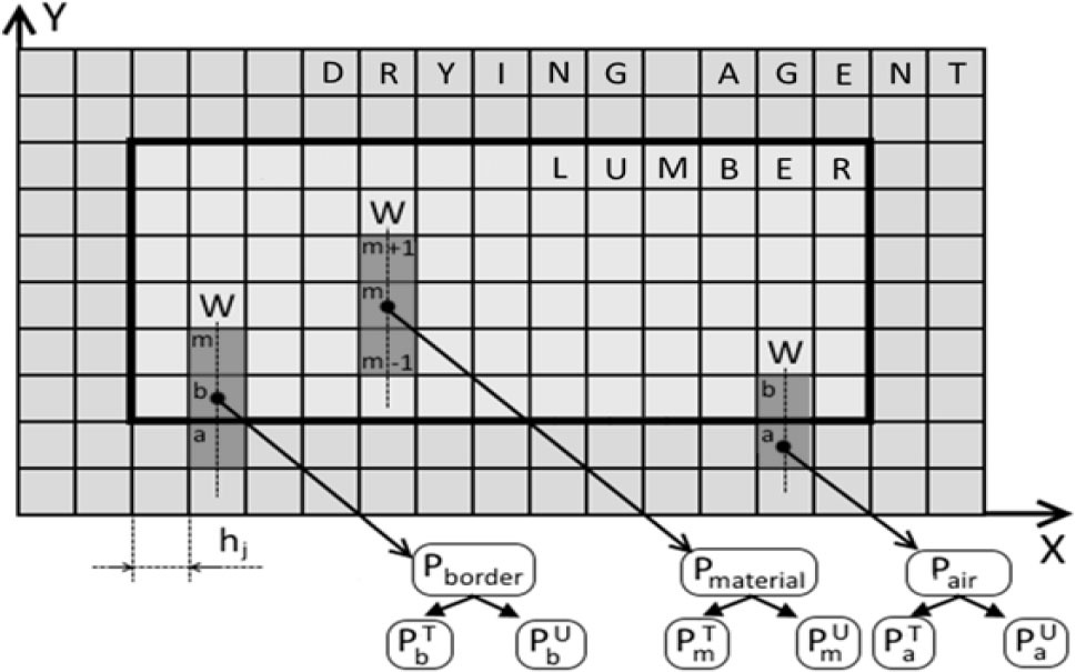
The program determines the type of each cell on the cellular automata field according to the algorithm (refer to Fig. 6).
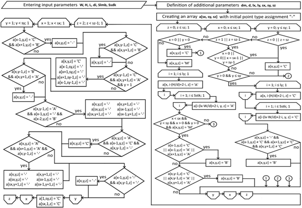
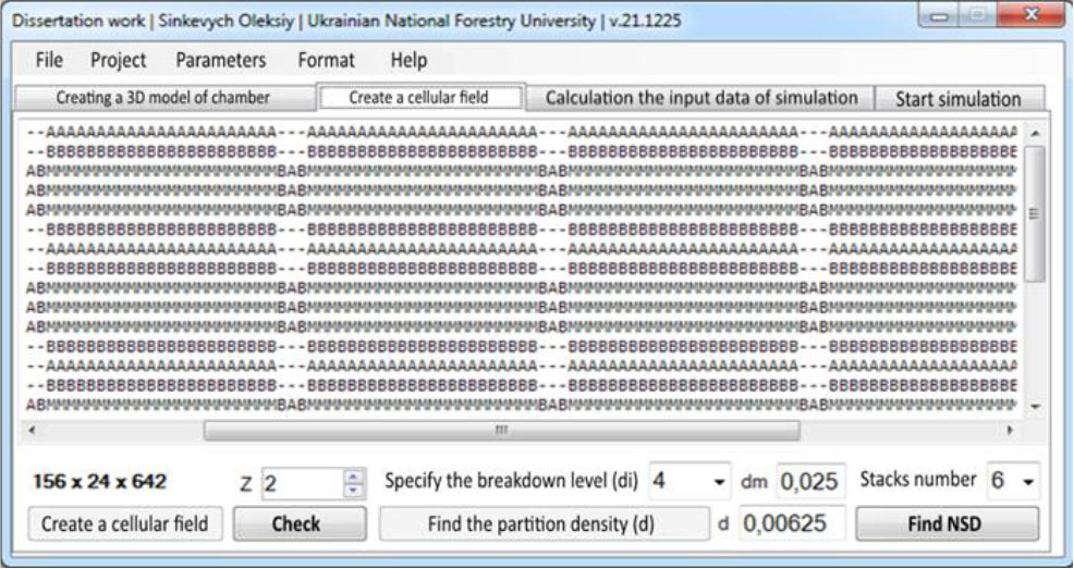
When considering the cellular automata field within the arrangement of the stacks, the cells can have different types, with the main ones being: “A” for the drying agent, “B” for the border of lumber, and “M” for their internal drying zone. To create a cellular automata field by using the software, it is necessary to open the second tab of the main program window (refer to Fig. 7). On this tab, users can inspect the structure of this cellular automata field. To do so, they need to specify one of the coordinates and click the “Check” button. The two-dimensional view of this field will be display in the window below.
The structure of each cell contains information about its moisture content, temperature, coordinates (location), and time. The inclusion of time allows for the observation of changes in all cell parameters over time, a crucial aspect when generating graphic dependencies for a specific cell. Simultaneously, the upper-left vertex of the selected cell determines the coordinates of its location.
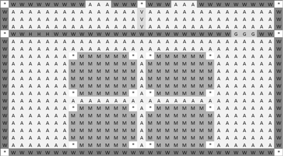
Considering the cellular automata field for the entire 3D model of the drying chamber, the cells have the following designations: “G” for the area of humidifying nozzles, “N” for the area of supply-exhaust channels, “V” for the area of axial fans, “H” for the location of water heaters, and “W” for the walls, ceiling, and chamber ceiling. These new designations enable the application of additional transition rules, particularly when the drying agent interacts with various components of the 3D model of the drying chamber. Such a cellular automata field is finite and constitutes one of the two parts of the cellular automata model. However, it’s crucial to consider the computational capabilities of computer equipment during its creation. Although fewer resources are utilized compared to the finite difference method (one cell replaces four points), the required resources for its creation remain substantial. Consequently, the constructed cellular automata field accurately replicates the assembly structure of the designed 3D model of the drying chamber (refer to Fig. 8).
ANALYSIS OF MATHEMATICAL MODELS OF HEAT AND MASS TRANSFER PROCESSES IN DRYING CHAMBERS
To create transition rules, it is imperative to initially analyze the pertinent mathematical models describing the heat and mass transfer processes during the drying of hygroscopic materials [10,11,12,13,14]. Those mathematical models must consider the impact of various components of the drying chamber on alterations in the parameters of the drying agent, as well as its influence on the dried material. Additionally, it is advisable to incorporate the influence of the temperature of the walls of the drying chamber and the heater on the temperature of the drying agent. Furthermore, it is crucial to consider the impact of humidifying nozzles on the relative humidity content of the drying agent. Another important task is involves determining the initial speed of movement of the drying agent, a parameter influenced by the characteristics of the axial fans and their quantity.
To modeling the drying process of hygroscopic materials, it is essential to consider the heat transfer among various components within the system. In this context, hygroscopic materials act as the heating object, with water heaters performing as the heat source. The drying agent enables the transfer of heat between them. Unfortunately, the walls, roof, and ceiling absorb a portion of the heat from the drying agent that has traversed from the heaters to the hygroscopic materials. Consequently, it is possible to make certain simplifications by treating all components contributing to heat loss as a unified entity, denoted by a general temperature, Tw. In essence, the heat exchange, as described above, incorporates the heat balance equation [15] for the heater, drying agent, and other components of the drying chamber, and taking the following form:
(1)
In turn, the moisture balance equation in the drying chamber [14, 15] can accommodate changes in the relative humidity of the drying agent, which changes with its temperature. Essentially, this equation can be formulated as follows:
(5)
According to the law of conservation of energy, the quantity of heat expended on heating and evaporating moisture from the hygroscopic material will always be equivalent to the amount of heat entering it [17]. For this, the heat balance equation within the hygroscopic material being dried can be employed, witch having the following form:
(7)
At the same time, the moisture content of the hygroscopic material being dried is determined as follows:
where: Lu – Luykov criterion, which reflects the ratio of the convective diffusion coefficient (am) to the heat diffusion coefficient (aq), Pn – Posnov criterion, which reflects the relationship between the intensity of thermodiffusion (δ∆Tm) to moisture diffusion transport (∆Um), KO – Kosovych criterion, which represents the dependence between the amount of heat expended on evaporating liquid from the hygroscopic material (r∆Um) to the amount spent on its heating C∆Tm, ε – phase transition coefficient.Thus, the aforementioned equations constitute a mathematical model of the heat and mass transfer process within the drying chamber. This model allows the determination of the relative humidity and temperature of the drying agent, along with the moisture content and temperature of the hygroscopic material. Similar to any mathematical model, it must incorporate boundary conditions. Given its intricacy, a dedicated diagram (refer to Fig. 9) was devised to illustrate the coordinates of all its borders.
Fig. 9.
The diagram illustrating the coordinates for the boundary conditions in the mathematical model
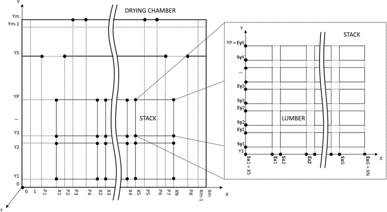
This diagram outlines the overall boundaries of the 3D model of the drying chamber. The X coordinate ranges from [0] to [Xm], and the Y coordinate ranges from [0] to [Ym]. The position of the supply and exhaust channels is determined by the Y coordinate [Ym], and X coordinates within [P3; P4] and [P5; P6]. The point [Ys] defines the location of the overlap along the Y coordinate. The diagram also illustrates the placement of side passages containing humidifying nozzles (on the right) and water heaters (on the left). These passages have fixed values, with the Y coordinate [Ys] and X coordinates within [P1; P2] and [P7; P8], respectively.
It is crucial to specify the coordinates of the stack locations, which can change, and their precise [Xn] and [Yp] coordinates can be determined when their quantity is known. The initial coordinates of the stack location always begin at [X1], and the end point of the X coordinate will be one step more [+1] than the starting point, for instance, [X2]. The height of one stack corresponds to the distance between points [Y1] and [Y2], while the distance between stacks is equivalent to the distance between points [X2] and [X3]. Similarly, the width of one stack is equivalent to the length of the interval [X1; X2].
The coordinates of the location points of hygroscopic materials within a specific stack can be determined using a similar principle. For instance, the starting coordinate of the material location always begins with “S,” and the ending one with “E.” The subsequent letter indicates the selected coordinate. Thus, one material has a height equivalent to the interval [Sy1; Ey1], and the width is equivalent to the interval [Sx1; Ex1]. Simultaneously, the height of one gasket between rows of hygroscopic materials is equivalent to the distance from point [Ey1] to [Sy2]. Therefore, to initiate the drying process (τ = 0), the following initial conditions, that characterizing the system’s initial state, are introduced and have the following form:
Due to the multitude of coordinates defining the locations of various boundaries, the 3D model segmented into three distinct zones, each with its specific set of boundary conditions. The first zone directly related to hygroscopic materials. It allows the determination of moisture content and temperature on the surface of a single hygroscopic material undergoing the drying process [12, 15, 16]. In this way, boundary conditions of this zone have the following form:
(9)
The second zone pertains to the positioning of the stacks, where the hygroscopic material undergoing drying exposed to its drying agent. Alterations in the relative humidity and temperature of the drying agent can be assessed within this zone [13,14,15]. So, the boundary conditions for this zone have the following form:
(10)
The last third zone encompasses the interaction of the drying agent with other components of the drying chamber. Within this zone, it is possible to determine the relative humidity and temperature of the drying agent at its various boundaries, such as those in contact with walls, heaters, supply and exhaust ducts, etc. Consequently, the boundary conditions for this zone take on the following form:
(11)
It is worth separately noting the influence of the number of axial fans and their power on the initial velocity of the drying agent. In this regard, it is important to consider the resistance of the stacks, which affects the initial velocity, and can be determined as follows:
where: Nst – total number of stacks, hst – height of one stack, lst – length of one stack, hg – height of the spacer between rows of materials in a stack, hw – height of one hygroscopic material, ec – coefficient of expenditure during the operation of fans, Pv – power of fan, Nv – number of axial fans, ν0 – initial velocity of the drying agent.DEVELOPMENT OF TRANSITION RULES FOR THE CELLULAR AUTOMATA MODEL
After analyzing the mathematical model, including its boundary and initial conditions, it becomes possible to formulate transition rules for the cellular automata model [17, 18]. The developed scheme (refer to Fig. 10) utilized to illustrate the conditional designations employed in these transition rules. It provides an example of the interaction among adjacent cells, where the interaction direction “W” corresponds to the Y coordinate.
In general, utilizing the cellular automata model involves the following steps:
− Establishing the direction of interaction “W” according to the normal distribution law;
− Start the iteration, equivalent to a time interval of ∆t seconds;
− Choosing the target cell (mc) following the uniform distribution law;
− Verifying the type of neighboring cell (nc) and applying the relevant transition rules;
− Repeating steps 2–4 until all cells are selected;
− Finalizing the execution of the current iteration and assessing termination conditions;
− Concluding the simulation if the test is successfully completed;
− Advancing the simulation time and returning to step one if the test not met.
A satisfactory condition to finish modeling is reaching the specified simulation time or the desired moisture content of the hygroscopic material undergoing drying. The main transition rules have the following form:
IF 'mc' = ≪M>
AND 'nc' = ≪M≫ AND
THEN
IF 'mc' = ≪M≫
AND 'nc' = ≪B≫ AND
THEN
IF 'mc' = ≪B≫ THEN
IF 'mc' = ≪A≫ AND 'nc' = ≪B≫ THEN
IF 'mc' = ≪A≫ AND 'nc' = ≪A≫ THEN
IF 'mc' = ≪A≫ AND 'nc' = ≪W≫ OR 'nc' = ≪V≫
THEN
IF 'mc' = ≪A≫ AND 'nc' = ≪H≫ THEN
IF 'mc' = ≪A≫ AND 'nc' = ≪N≫ THEN
IF 'mc' = ≪A≫ AND 'nc' = ≪G≫ THEN
Where the value of coefficients C1–C15 can be calculated as follows:
where: hs – distance between hygroscopic materials in a stack and the gap between two stacks, CC – specific heat capacity of the condensate, ρC – density of the condensate, δ – thermal gradient coefficient, ρm – density of materials, cm – specific heat capacity of materials, λj – thermal conductivity coefficient of the material in the specified direction, hj – size of one cell, ∆t – time for one iteration. The value of j can be “1” for “x” and “2” for “y”.DEVELOPMENT OF THE DATABASE AND DISTRIBUTION OF ACCESS RIGHTS
To enter the input data of the simulation, it is necessary to open the third tab of the software (refer to Fig. 11).
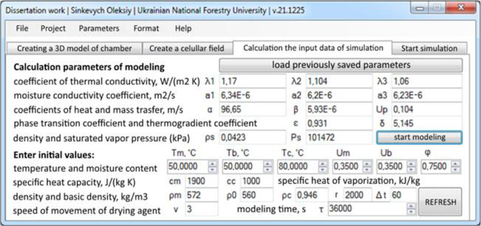
On this tab, the user enters the initial values of some parameters, in particular: temperature and moisture content of lumber; temperature and relative humidity of the drying agent; specific heat capacity; density and basic density of the material; specific heat of vaporization; simulation time and time step. At the same time, the rest of the parameters, most of which are represented by different coefficients, will be determined automatically. Having all the parameters for the simulation, user can start its execution using the same tab.
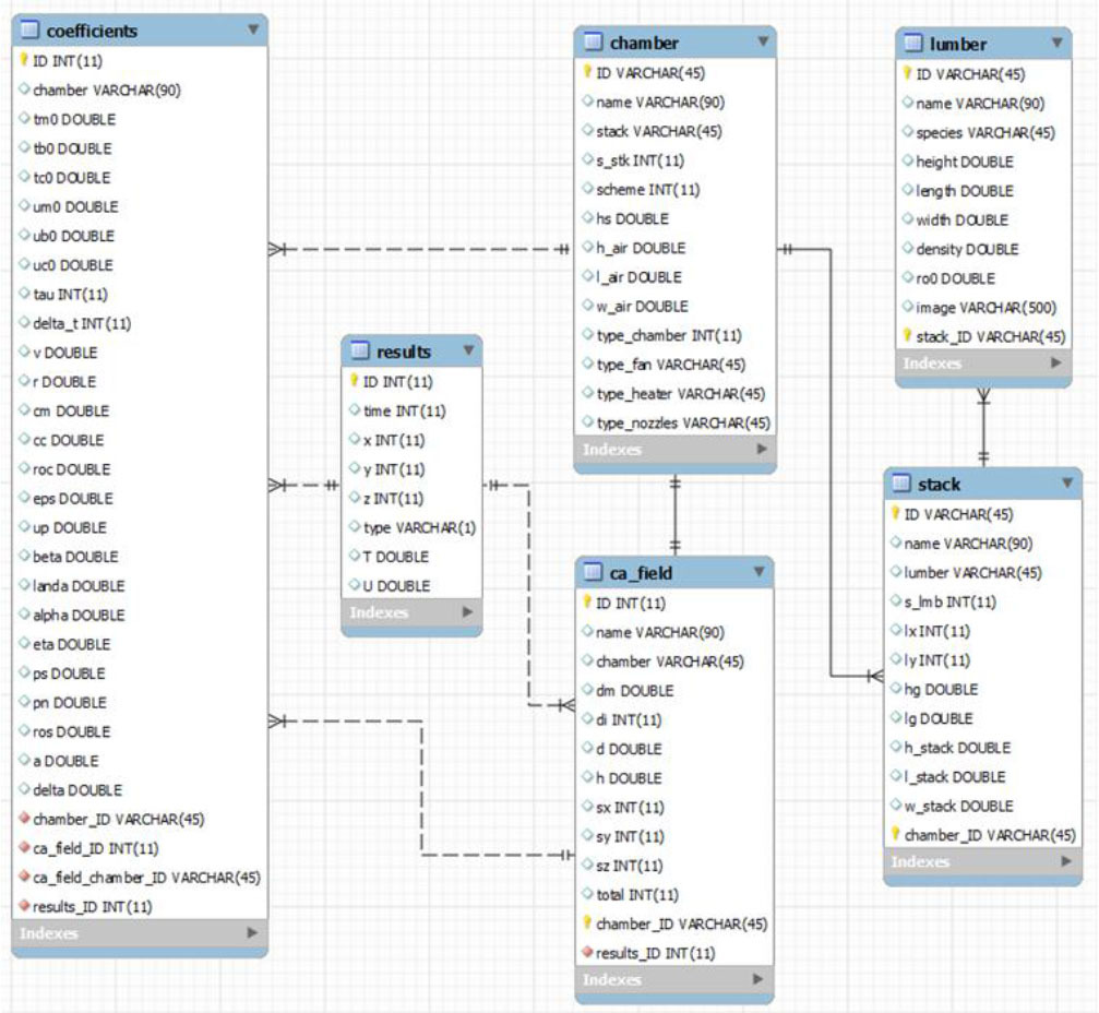
To carry out modeling, it is absolutely necessary to have a database in which the results will be stored. To create it, it was decided to use the MySQL Workbench Community Edition environment. The created database is named “dissertation” and consists of several interconnected tables, namely: “lumber”, “stack”, “chamber”, “ca_field”, “coefficients” and “results”. The “lumber” table contains a unique lumber code that is generated automatically and has the following structure: “ХХ.LL.HH.WW”, where “ХХ” is the type of wood (birch - “BR”, cedar - “CD”, Beech - “RT”, maple - “MP”, oak - “OK”, pine - “PN”, teak - “TK” and other), “LL” - length, “HH” - height, “WW” - width of lumber in mm. Also in this table there is information about the density of the material. The “stack” table contains a unique stack code that is generated automatically and has the following structure: “XX x LL”, where “XX” is the number of lumber in the stack, and “LL” is the unique lumber code. Also, this table contains data on the number of lumber in the stack, their location, and information on the size and number of spacers between rows of lumber. The “chamber” table contains the unique code of the drying chamber, which is generated automatically and has the following structure: “ХХ→SS”, where “ХХ” is the number of stacks in the drying chamber, and “SS” is the unique code of the stack. Also, this table contains information about the number of stacks in the chamber and the scheme of their arrangement along it. The “ca_field” table contains information about the cell autofield, including the number and sizes of cells. The “coefficients” table contains information about all modeling parameters, both initial, which are constant, and current, which change with the passage of model time. The last table “results” contains information about the results of the simulation and is the largest among all of them. To display the entities, attributes and relationships between them, an Entity-Relationship (ER) diagram (refer to Fig. 12) was created. It provides an opportunity to better understand how the data will interact with each other in the developed software.
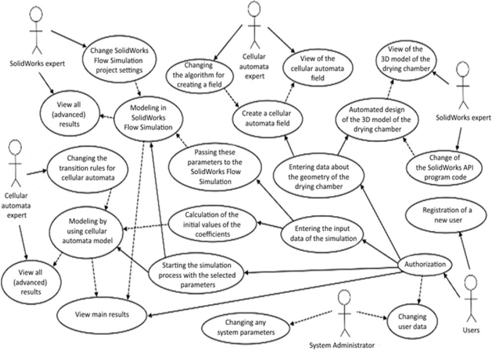
To visualize the functionality of the system from the perspective of users and other system agents, a UML use case diagram was created (refer to Fig. 13). It is used to describe how a system interacts with its environment, including users and various processes. By its structure, this diagram has actors that interact with the system. These actors are divided into 4 types, namely “Users”, “SolidWorks experts”, “Cellular automata experts” and “System administrators”. Each of them has its own access rights and certain usage options. Each of these use cases represents a specific scenario that the system supports and can implement. At the same time, each scenario details the sequence of actions and interaction between actors and the system.
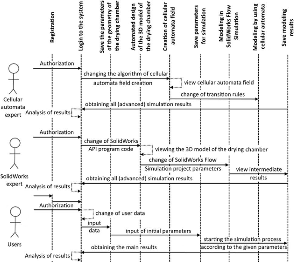
To visualize the interaction between system components within a specific usage scenario, a sequence diagram was created (refer to Fig. 14). It helps to understand the sequence of actions and the exchange of messages between different elements of the system involved in a specific process. In turn, this diagram shows three actors and their sequence of actions in the system.
SIMULATION OF THE DRYING PROCESS OF HYGROSCOPIC MATERIALS USING THE CELLULAR AUTOMATA MODEL
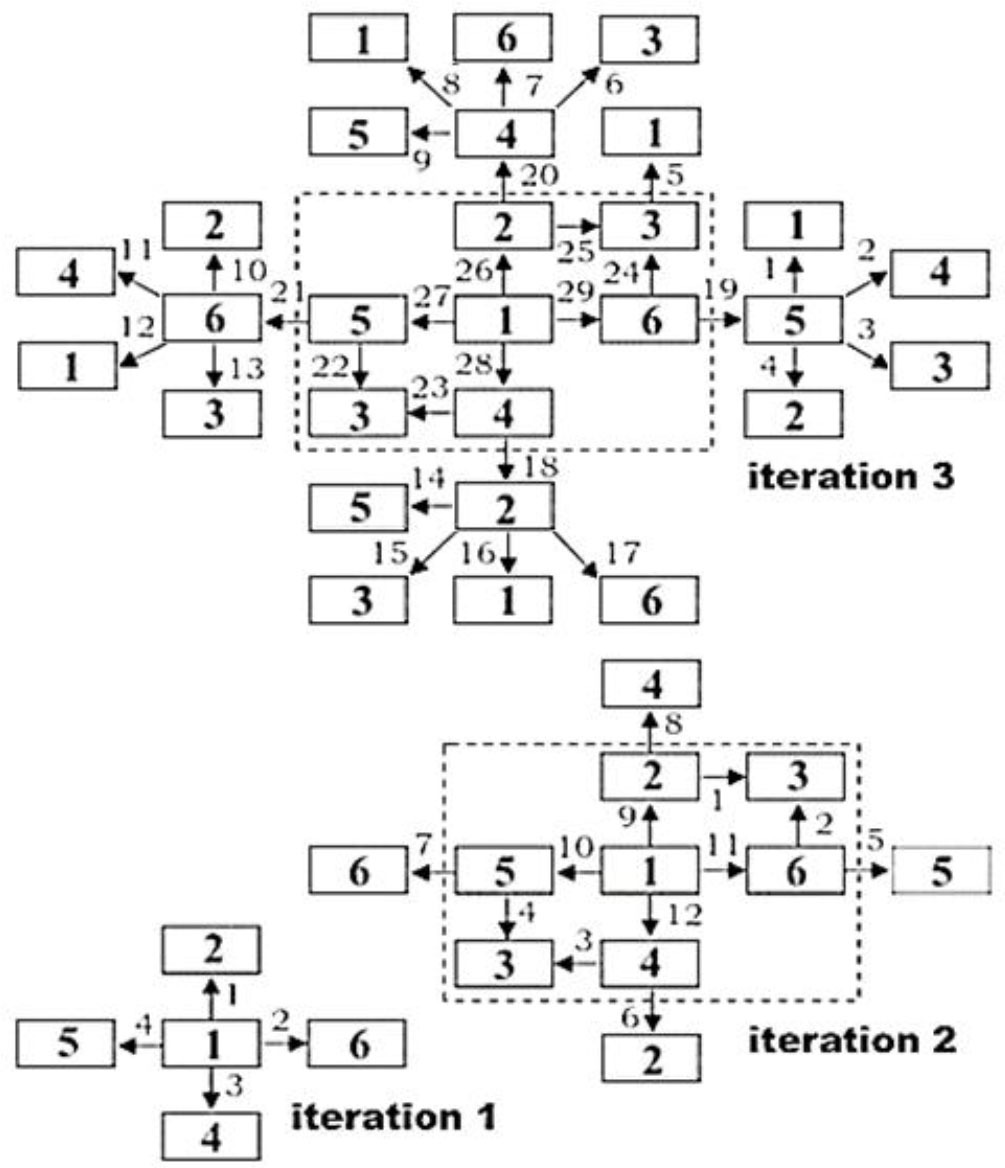
After initiating the simulation, an iterative cycle begins, executing transition rules among closely located cells. Through these interactions, the key parameters of both the drying agent and the hygroscopic material undergo changes. As illustrated in Fig. 15, influencing a single cell leads to subsequent alterations in 27 cells after several iterations. This approach effectively illustrates the cellular automata principle [18], where modifying values in specific cells, such as on material surfaces, directly influences internal cell values. To conveniently monitor temperature and moisture content changes in the drying material, users can utilize the “View values” window located in the “Format” section of the software’s main menu.
This window helps user to view the changes of parameters in two-dimensional space on the cellular automata field, but for this, they need to specify the starting point of the tracking according to the coordinates (lower left corner of the field). After that, user can see cells that display a given parameter to choose from (temperature or moisture content). For the convenience of obtaining graphical dependencies, the values of the main parameters displayed in the right part of the window. At the same time, user can select a specific area on the cellular automata field, thus obtaining the value of the desired parameter in space and time.
ANALYSIS OF THE OBTAINED SIMULATION RESULTS
As a result of the simulation [19], graphical dependences of the main parameters of the hygroscopic material to be dried and the drying agent over time were obtained (refer to Fig. 16 and 17). The main parameters include: the average relative humidity of the drying agent (
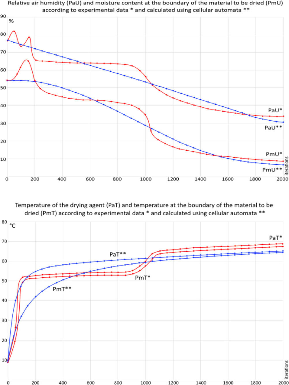
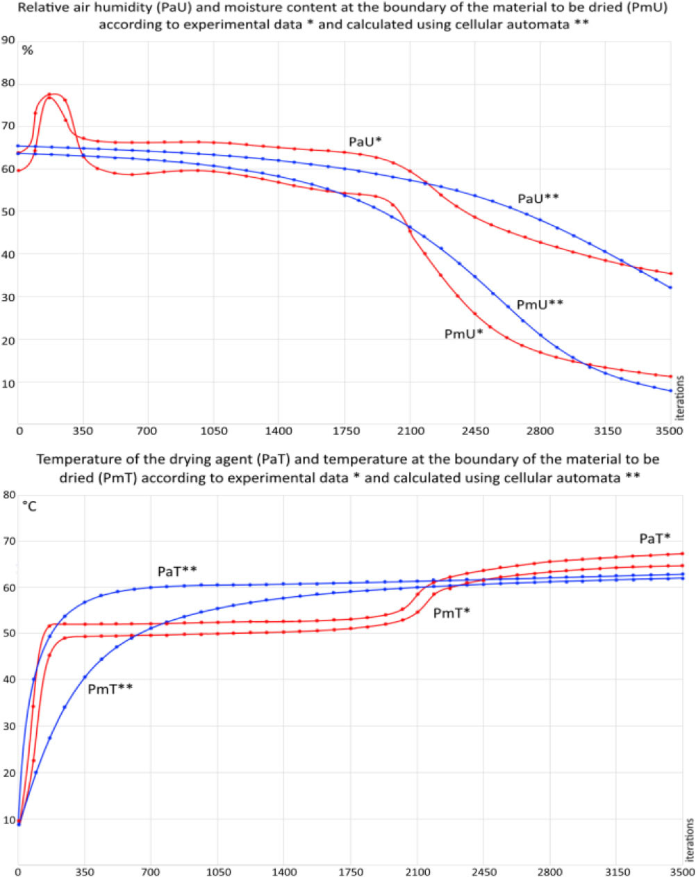
To verify the obtained results, they compared with experimental data that obtained using the “LK-ZDR-100” wood drying chamber, located at “Rodors” LLC (Khmelnytskyi region, Ukraine). Data for compared the first study collected using sensors between 29/10/18 and 06/11/18 for 30 mm thick pine material with an initial moisture content of 55%. Data for compared the second study collected between 18/03/23 and 01/04/23 for 45 mm thick pine material with an initial moisture content of 65%.
The input parameters for comparing the results are as follows: initial relative humidity of the drying agent is 77% / 74%, the temperature of the heat carrier (hot water in the heaters) is 70 °C (for both data sets), the initial temperature of the drying agent is 15 °C / 19 °C, the initial temperature on the surface of the hygroscopic material is 13 °C / 18 °C, the simulation time is 166 h / 291 h, and the iteration step is 300 s (for both data sets).
Visual evaluation of the results is important, but it doesn’t provide a way to determine the accuracy of the modeling. In general, there are many ways to determine accuracy, each of which depends on the context and specifics of the comparative data [20]. In this case, two of the most common methods chosen to assess the accuracy, namely, the mean absolute error (MAE) and the mean absolute percentage error (MAPE). As a result of the calculations, the values of these errors were determined for the temperature and humidity parameters of the drying agent and hygroscopic material for both data sets.
It was established that the average value of MAPE is 13%. The largest values amounting to approximately 24%. This result may indicate that a limited number of cells of cellular automata field and limited transition rules between them were used in the initial phase of the simulation. Over time, the number of cells increases and the accuracy of the results improves significantly. Therefore, MAPE at the end of the simulation doesn’t exceed 9%. This analysis confirms the accuracy and correspondence of the obtained results to real drying conditions. In addition, simulation results can be used to determine optimal input parameters for simulation in computational fluid dynamics programs, including SolidWorks Flow Simulation.
In general, the topic of this research is new. In this regard, the research results can be compared with related works of other authors, in particular, in work [3]. In this work, a three-dimensional mathematical model of heat and moisture transfer during drying of wood in drying chambers was developed. This model was successfully verified using numerical simulations and experiments, including the analysis of air movement and moisture. In turn, in [4] heat and mass transfer in the process of high-temperature processing of wood were analyzed. It allows to evaluate the relationship between changes in temperature and moisture content in wood in its drying agent. In addition, some authors [21, 22] also use the capabilities of automated design when performing a related class of tasks. To conduct similar research, some authors also resort to the use of cellular automata models [7].
CONCLUSIONS
To summarize, this study makes a significant contribution to the field of CAD design of 3D models of drying chambers by using tools for parameterizing its geometric characteristics. At the same time, the proposed model of cellular automata provides an effective tool for modeling the drying process of hygroscopic materials in such designed 3D models of drying chambers.
The key achievement of this work is the integration of the algorithms for automated 3D design and the cellular automata model. Therefore, the developed software not only simplifies the design process, saving precious time and material resources, but also provides a powerful platform for modeling and studying the dynamics of heat and moisture transfer during the drying of hygroscopic materials.
The validation of the developed cellular automata model was carried out by comparing the obtained results with experimental data, with the average MAPE value not exceeding 13%. This level of error is acceptable, since the processes of heat and mass transfer during the drying of hygroscopic materials characterized by complexity, multifactoriality, and nonlinearity. This makes modeling with absolute accuracy impossible, even with the most advanced approaches. Under such conditions, an error of 15% considered typical for most models in this field, since achieving perfect accuracy is extremely resource-intensive. At the same time, the proposed cellular automata model demonstrates accuracy comparable to existing models, but characterized by higher computational speed, which makes it practically valuable for real-world applications.
It is also worth noting the possibility of determining changes in the parameters of the hygroscopic material and its drying agent during the modeling process. This was realized due to the improved structure of the cellular automaton field, which takes into account the physical and geometric characteristics of the whole 3D model of the drying chamber. This field structure makes it possible to use different types of cells and the relationships between them, which are realized by the corresponding transition rules.