INTRODUCTION
Within intralogistics automation, line-following robots facilitate routine material moving along defined trajectories, meeting stringent requirements for operational precision and reliability. These systems also allow for flexible path adjustments to accommodate changes in facility layouts. Their ability to accurately follow predefined paths makes them valuable for logistics, industrial production lines, educational competitions, improving efficiency and reducing operational costs Furthermore, the integration of advanced measurement systems into autonomous guided vehicles (AGV) has become a cornerstone for achieving precision in factory logistics [1].
Traditional line following robots often rely on infrared or reflective sensors. However, these sensors exhibit limitations in environments with low contrast, dust or external interference [2]. While infrared sensors are cost effective, their reliability is frequently compromised by surface reflectivity and ambient noise, necessitating more sophisticated optical measurement techniques [3-7]. Recent research suggests using cameras instead of infrared sensors to overcome these limitations, enabling more accurate line detection and even obstacle recognition. Image processing and computer vision algorithms enhance the robot’s flexibility and stability, especially in complex or blurred path conditions [8-11].
Although camera systems offer numerous advantages, image acquisition is susceptible to light interference. In environments with dynamic lighting such as those with high-intensity light, low light, or shadow line identification becomes challenging. Light interference directly impacts image contrast, degrading the performance of edge detection algorithms like the canny filter [12-14]. Recent advancements in image enhancement have highlighted that automatic non-linear mapping is essential for robust feature extraction in high dynamic range environments [15]. Additionally, strong light shining directly on the line can cause the line to disappear, leading to the camera not being able to capture the line and resulting in inaccurate robot movement [16].
To overcome the issues, the gamma correction algorithm has been proposed as a solution to adjust the brightness and contrast of an image from a camera [15]. Gamma correction is a technique that helps adjust brightness by applying a non-linear function to adjust the light or dark levels of an image [15,17]. If the ambient light is too strong, the gamma correction algorithm will adjust the input image reducing contrast and brightness. After gamma correction, the image will show clear details on the line [18,19]. However, ensuring stable and precise movement in real-world environments remains a formidable challenge. Paths in practical applications rarely limited to straight lines; they often consist of intricate curves and deviations ranging from 0o to 180o [20]. Without precise speed modulation, a mobile robot is prone to losing track of the line, especially when encountering sharp turns or variable lighting conditions. Traditional control methods, such as proportional-integral-derivative controller, rely heavily on exact kinematic models, which frequently fail to account for the non-linear dynamics and external noise inherent in physical environments [21]. Therefore, fuzzy logic controller (FLC) has emerged as a robust alternative. FLC excels in managing non-linear systems and environmental uncertainties by incorporating human-like reasoning. These studies demonstrate that fuzzy inference systems can significantly improve path-tracking stability and reduce oscillations compared to classical methods [22-25]. Furthermore, experimental evidence confirms that vision-based fuzzy systems provide superior adaptability to visual noise, ensuring smoother transitions through curved path segments.
This study proposes a specialized vision-based fuzzy control framework for AGV in complex industrial environments. The controller utilizes a Mamdani inference system to map two primary visual inputs the relative deviation angle (θ) and the horizontal central coordinate (Cx) into pulse width modulation (PWM) signals for the drive motors. While vision-based fuzzy control is established, existing systems predominantly rely on high-end edge computing to minimize latency and require strictly controlled lighting. To enable robust deployment on resource-constrained, low-cost hardware under variable conditions, this paper makes the following contributions: (i) by synergistically combining dynamic gamma correction with Otsu’s thresholding, the system optimizes image contrast to ensure reliable path extraction under fluctuating light intensities, overcoming the brittleness of static vision algorithms; (ii) the proposed rule base and membership functions are explicitly designed to suppress oscillations and maintain stable tracking despite the inherent communication and processing delays of wireless vision modules.
The remainder of this paper is organized as follows: Section 2 details the system architecture, image processing algorithms incorporating gamma correction and the design of the Mamdani FLC. Section 3 evaluates the system’s performance through experimental validations under varying illumination and trajectory conditions. Finally, the key findings and outlines potential directions for future research and optimization are summarized in section 4.
METHODOLOGY
Design of the adjustment mechanism
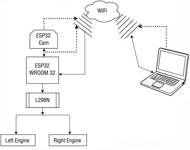
The hardware architecture and integrated control loop of the system are depicted in the block diagram in Fig. 1. The system is executed in accordance with the loop vision-based control model. In this investigation, the ESP32-CAM module [26] was utilized and configured for a resolution of 320*240 pixels. This constitutes the appropriate configuration to ensure that the input image possesses sufficient detail for subsequent processing phases, while not overburdening the data transmission bandwidth and off-board processing velocity on the computer. Consequently, the system can sustain acceptable loop latency, which enhances the stability, reactivity of the controller in acceptable latency. The configuration is predicated upon a centralized data processing framework (off-board processing), which commences with the acquisition of unprocessed images from the sensor and its instantaneous transmission via Wi-fi protocol to the workstation computer. This paradigm facilitates the transference of computationally demanding tasks such as gamma correction algorithms [27], and image conversion pipelines to high performance processors, thereby fundamentally surmounting memory and processing capacity constraints on embedded microcontrollers.
The raw input image data is initially subjected to preprocessing via the gamma correction algorithm to normalize and enhance contrast, thereby ensuring feature detection robustness under dynamic lighting conditions. Subsequently, the system executes a feature extraction process to delineate the path contours. The resulting geometric parameters specifically Cx and θ are then fed into the FLC [28]. The final execution phase of the system architecture entails the transmission of control signals back to the ESP32 WROOM 32 module. Based on the computational outputs of the FLC, corresponding PWM signals are generated to regulate the L298N motor driver [29]. The independent modulation of power supplied to the two motors enables precise steering manoeuvres and speed control, thereby maintaining a stable trajectory.
Image processing algorithms
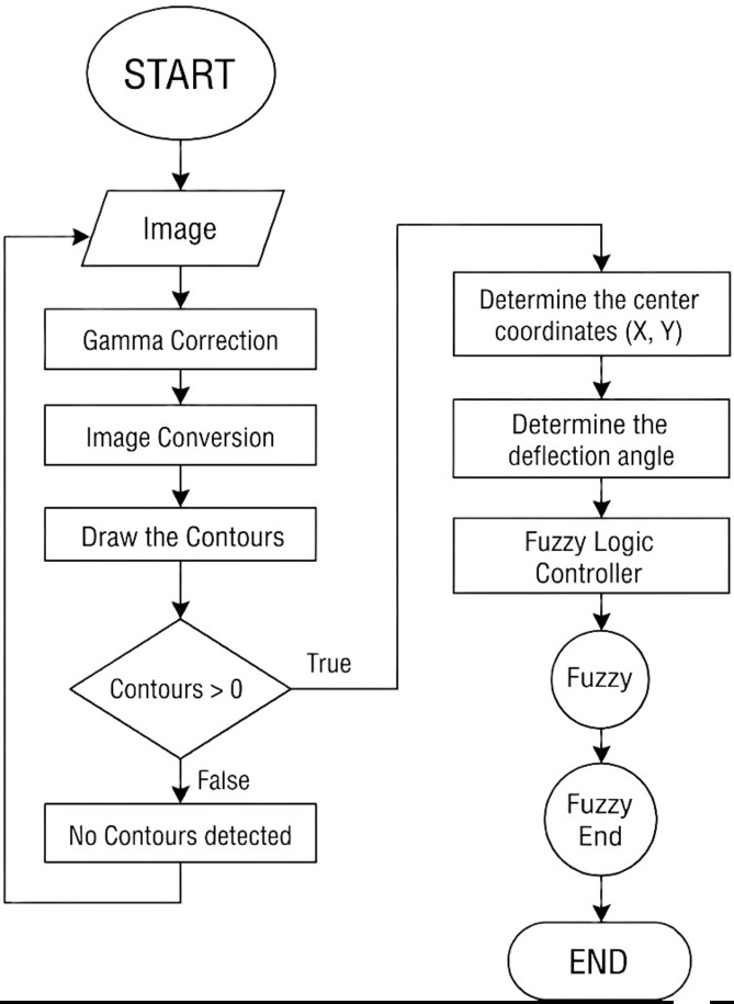
The flowchart depicted in Fig. 2 delineates the progression of data processing commencing from the acquisition of raw signals through to the implementation of guidance control. The procedure is initiated through the continuous capture of images via the camera module, which is subsequently followed by a preprocessing phase utilizing the gamma correction algorithm. This normalization process is pivotal in achieving contrast balancing, thereby establishing the foundation for image segmentation and contour extraction, which are critical for the precise delineation of the moving trajectory amidst the background noise under fluctuating lighting conditions. During the contour verification phase, if no valid features are detected, the system enters a standby state to prevent erroneous displacement and overshoot.
Conversely, upon validation of a trajectory, the algorithm performs geometric estimation to derive two critical parameters: the centroid coordinates (x, y) and the heading θ. These values serve as crisp inputs for the FLC. The fuzzy inference system processes these spatial variables to modulate the appropriate PWM signals for the motor drivers. This control architecture establishes a loop feedback mechanism.
Gamma correction
Gamma correction is a pixel intensity transformation technique based on a power law function, playing an important role in compensating for the non-linear characteristics of the image acquisition process and enhancing local contrast [24]. This operation follows the fundamental power law relationship defined:

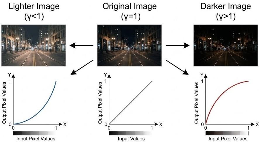
where: Iin denotes the normalized input intensity, Iout the output intensity, and γ the gamma parameter. For 0 < Iin < 1 when γ < 1 the mapping increases pixel intensity values and thus brightens the image, enhancing details in dark regions; when γ > 1 it decreases pixel values and therefore darkens the image, compressing intensities in bright regions; when γ = 1 corresponds to an identity mapping. In accordance with equation (1), the input pixel intensities, initially defined within the 8-bit range [0, 255], are normalized to the unit interval [0, 1] as illustrated in Fig. 3. The selected gamma coefficient is applied to modulate the luminance profile. The output is finally rescaled to original [0, 255] domain.
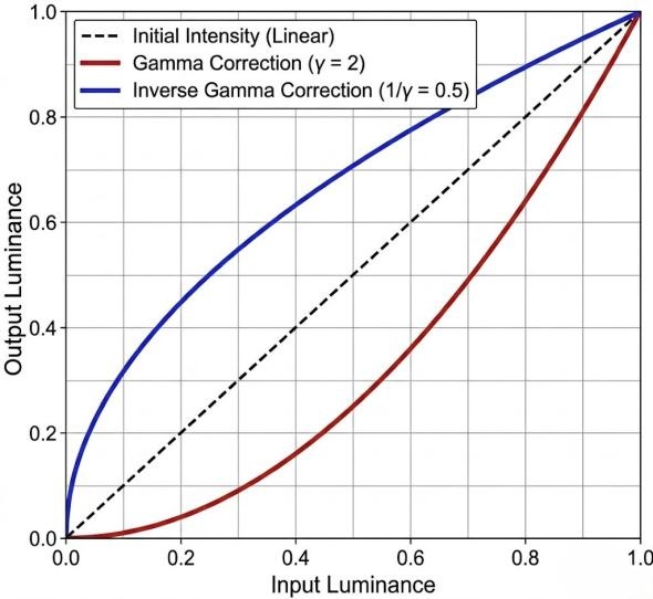
The proposed system employs an automatic inverse gamma compensation mechanism. Instead of relying on empirical para-meters, the gamma coefficient γset, is dynamically estimated for each frame based on the mean grayscale intensity (μ) of the camera’s view [30]:

where ϵ is a small constant to prevent division by 0. To mitigate extreme noise amplification in severely dark or overexposed environments, the calculated γset is constrained within an operational bound of [0.5, 2.8]. The formula after applying automatic inverse gamma and the effective exponent will be:


Consequently, the operational logic is defined as follows: when γset > 1, the effective exponent becomes less than 1 (1/γset < 1). This results in a logarithmic-shaped curve that brightens the image, enhancing details in shadowed areas (illustrated by the red line in Fig. 4); when γset < 1, the effective exponent becomes greater than 1. This darkens the image to mitigate overexposure.
The preceding gamma correction stabilizes the local contrast, ensuring the grayscale histogram maintains a distinct bimodal distribution in environmental illumination changes. This ensures a well-defined global maximum for the inter-class variance, enabling Otsu’s algorithm of the next step to reliably extract the optimal threshold T without manual parameter tuning.
Preprocessing and binarization
The image is converted to a single channel grey scale representation to reduce computational complexity while preserving luminance information for exploiting intensity cues that discriminate the guidance line from the background. Grayscale intensity is a necessary factor for the binarization step and directly affects the accuracy of subsequent contour-based detection of the guidance line. To prepare the input data for the visual processing module, this study employs a colour to grayscale conversion method based on the ITU-R BT.601 recommendation [31]. This approach assigns a prioritized weight to the green channel, aligning with the characteristics of image sensors utilizing a Bayer matrix, where in the green channel typically possesses a higher sampling density and a lower noise floor compared to the remaining channels. Consequently, this grayscale projection optimizes the signal to noise ratio and preserves critical edge features, thereby enhancing the reliability of subsequent binarization and contour detection stages relative to simple arithmetic averaging. Specifically, for an 8-bit image where R, G, B ϵ [0, 255], the grayscale value is computed as follows:

After inverse gamma enhancement and grayscale conversion, the image is binarized using an automatic global inverse binary threshold to separate the guide line (foreground) from the background. Let Igrey (x, y) ϵ [0, 255] denote the 8-bit grayscale intensity at pixel (x, y). The binary image Ibin ϵ (x, y) is obtained via inverse binary thresholding equation:

here, the binarization threshold T isn’t fixed, the dynamic threshold T is calculated using Otsu’s method by maximizing the inter-class variance between the background and the guidance line [32]:

where ωo(t) and ω1(t) are the cumulative probabilities of the two classes separated by threshold t, and μo(t) and μ1(t) are their respective mean intensities.
The inverse thresholding mode is adopted so that pixels belonging to the guidance line are mapped to the foreground (high intensity, 255), while the background is suppressed to 0. This representation is convenient for the subsequent contour-based processing, as it yields a clean foreground mask from which the dominant path contour can be extracted.
Path parameters estimation
This study utilizes PCA on a set of image pixels belonging to the track’s boundaries to extract two core control parameters cross-track error and heading error [33]. The cross-track error is represented by the lateral centroid position relative to the image centre. The system operates in a standard image coordinate, where the origin (0,0) is located at the top left corner of the image frame, the X-axis points to the right and the Y-axis points downwards. Therefore, the robot’s forward motion (towards the top of the image) corresponds to the negative direction of the Y-axis. The standard direction of motion for the robot is along the Y-axis, corresponding to the unit vector ĵ = (0, –1). The ideal centre line lies in the middle of the field of view along the X-axis, with the coordinate Xref = W/2 (where W is the width of the image). The system identifies a discrete set of N points belonging to the two boundaries of the track. Let 𝒫 be the set of coordinate vectors for these points:

The cross-track error evaluates the translational displacement of the robot relative to the track’s centre, reflecting the degree to which it has slipped from the intended trajectory. The centroid (C̄x, C̄y)T of the point set 𝒫 is calculated as the expectation:

The heading error evaluates the relative angular deviation between the robot’s longitudinal axis and the tangent of the road ahead. PCA is applied to find the axis of maximum variance regarding the track’s morphology, shifted the origin to the centroid C to eliminate the translational component. The 2×2 covariance matrix C is defined as:

To obtain the maximum eigenvalue λmax (representing the longitudinal spread of the track), we solve the characteristic equation (C – λI) = 0 and solve the equation Cv = λmaxv to find the corresponding eigenvector v = (vx, vy)T. The PCA algorithm returns an eigenvector v that lies on a line but has an ambiguous direction. Since the robot’s forward vector aligns with the upward direction of the image frame (where Y-axis values decrease), the y component of the directional vector must be strictly negative (y < 0). The normalized directional vector v* is determined by the conditions:

Then, the deviation angle θ is calculated relative to the positive X-axis. Since the standard image coordinate system employs a downward-pointing Y-axis, the component is inverted to map the directional vector back to standard cartesian trigonometry. Consequently, the angle θ (in degrees) is derived as follows:

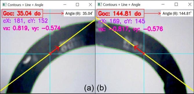
Based on this formulation, the path direction is classified as follows: (i) if > 0 0o < θ < 90o the track diverges to the right relative to the camera’s field of view, requiring the controller to execute a right turn; (ii) if < 0 90o < θ < 180o the track diverges to the left, requiring the controller to execute a left turn; (iii) if = 0 (and < 0) θ = 90o the robot is moving approximately parallel to the track centre line. The practical outcome of this angular estimation, illustrating both rightward and leftward deviations on the image frame, is depicted in Fig. 5.
Fuzzy logic controller design
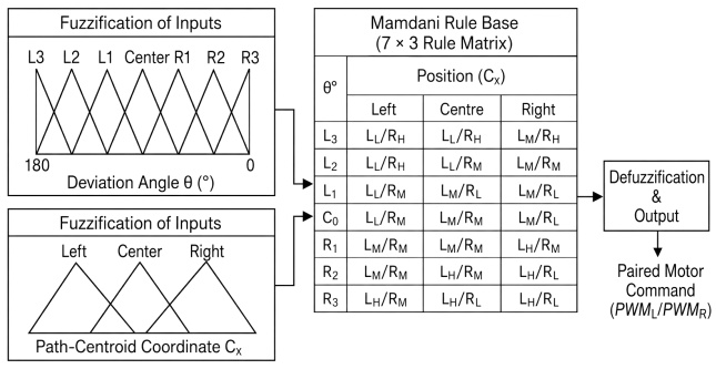
The FLC architecture is designed as a coupled multi-input multi-output (MIMO) system, comprising three primary stages: fuzzification, the fuzzy inference engine, and defuzzification. Fig. 6 illustrates the overall structure of the proposed FLC. The fuzzy inference engine simultaneously processes two fuzzified visual inputs (θ and Cx) through a unified Mamdani rule base to directly generate left pulse width modulation (PWML) and right pulse width modulation (PWMR) for two independent wheels.
Fuzzification
The system processes two inputs derived from the vision module: the centroid coordinate (Cx) and the angular discrepancy (θ) - which is defined as the angle between the robot’s current heading and the tangent of the target path. In this study, triangular membership functions are employed to fuzzify the data, where the lateral position Cx is mapped into three sets: left, centre and right to determine the robot’s offset relative to the path centre (Fig. 7b).
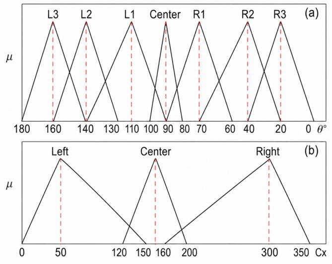
For θ, the range from 0° to 180° is discretized into seven levels as L3, L2, L1, C0, R1, R2, R3 (as Fig. 7a). This data granularity allows the controller to distinguish between minor steering errors and sharp turns. The resulting membership grades serve as the antecedents for the Mamdani inference rules, mapping the input pair (θ, Cx) to the corresponding motor commands.
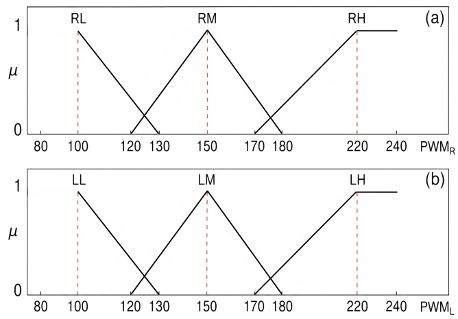
Motor speed control signals are categorized into three output PWM levels: left low (LL), left medium (LM), left high (LH), right low (RL), right medium (RM), and right high (RH). To facilitate defuzzification, these variables are represented by fuzzy sets within the drive system’s PWM domain. Fig. 8 details the membership functions for PWML and PWMR, defining the specific control levels activated during the inference process. These signals are ultimately aggregated and converted into crisp PWM values to command the two motors.
The output membership functions of PWMR (Fig. 8a) and PWML (Fig. 8b) within the effective PWM operating range of the drive motors (PWM ≥ 100). Specifically, the minimum output sets, RL and LL, are modelled as left-shoulder functions with approximate parameters (100,100,130). This prevents the low-speed output sets from extending into ineffective PWM regions that may not ensure stable motor rotation; the medium output sets, RM and LM, are defined as triangular functions over (120,150,180); and the maximum output sets, RH and LH, are modelled as right-shoulder functions, increasing from PWM = 170 and reaching full membership at PWM ≥ 220. This arrangement provides smoother and more stable defuzzified PWM commands in the extreme control regions.
Fuzzy rule base
Following the fuzzification of the input variables (θ and Cx), the Mamdani inference engine executes the fuzzy rule base to compute the corresponding motor control commands (PWML and PWMR). The rule matrix is derived from the differential drive kinematics of mobile platforms [34]. This approach establishes a proportional steering gradient, converting spatial deviations into velocity differentials between the robot’s two wheels.
The fuzzy rule matrix is organized into a 7×3 structure to simultaneously coordinate motor control commands based on combinations of the yaw angle and position fuzzy sets. These rules are designed such that every input combination results in a deterministic pair of the outputs. Details regarding the coordination rules for each operating scenario are summarized in Tab. 1.
Tab. 1.
Rule matrix of the fuzzy inference system for left/right motor control
| Angle (θ) | Position (Cx) | ||
|---|---|---|---|
| Left | Centre | Right | |
| L3 | LL & RH | LL & RH | LM & RH |
| L2 | LL & RH | LL & RM | LM & RM |
| L1 | LL & RM | LM & RL | LM & RL |
| C0 | LL & RM | LM & RM | LM & RL |
| R1 | LM & RM | LM & RM | LH & RM |
| R2 | LM & RM | LH & RM | LH & RL |
| R3 | LH & RM | LH & RL | LH & RL |
Technically, θ provides predictive data on positional trends, enabling the controller to execute rapid steering adjustments to align the robot’s heading parallel to the reference path. Prioritizing the processing of theta allows the system to respond quickly to abrupt changes in trajectory curvature.
Meanwhile, Cx serves to correct positional errors and maintain system stability and minimize oscillations. In feedback controllers, focusing solely on angular adjustments often causes the robot to intercept the reference line at high angular velocities, leading to overshoot and continuous sinusoidal oscillations around the path. In this context, Cx acts as a modulating the turning intensity based on the actual lateral distance to the centre line.
This integration creates a control mechanism that balances directional response speed (governed by theta) and positional stability (maintained by Cx). This results in a smoothed trajectory and ensures the robot converges stably toward equilibrium, preventing uncontrolled oscillations and overshoots caused by transmission delay.
Fig. 9 illustrate the response surfaces of the PWML and PWMR outputs, respectively. These surfaces represent the nonlinear mapping between the input state variables and the control signals of the two motors. Although based on the same set of input state variables, the two response surfaces of PWML and PWMR are established independently. This characteristic allows the controller to perform flexible differential responses, increasing the robot’s manoeuvrability in various scenarios.
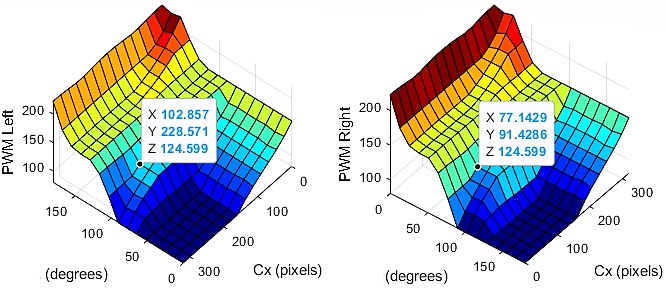
The continuity of the surfaces ensures that the control signal changes smoothly across the entire domain of theta and Cx values. This prevents abrupt transitions and wobbling when the robot changes operating states in sharp turning scenarios. At a given time, the difference in slope of each independent surface determines the degree of PWM difference between the two wheels. That provides the necessary torque to steer the robot’s movement.
EXPERIMENTAL RESULTS AND DISCUSSION
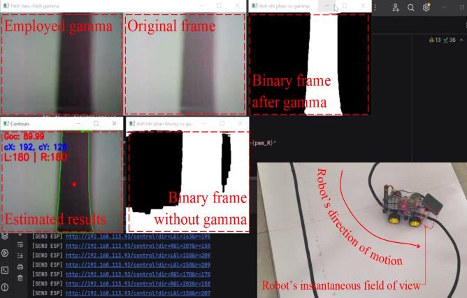
This section evaluates the proposed vision and control pipeline under varying illumination and trajectory conditions, focusing on segmentation quality and loop steering reliability. The evaluation is carried out on the physical prototype shown in Fig. 10. Track images are captured by the camera and delivered to a host computer via Wi-Fi. The centroid coordinate (Cx) and the angular discrepancy (θ) are estimated from each frame. The computed control commands are then transmitted back to the embedded controller to regulate the two guiding motors of the robot.
Image processing under illumination variations
The effectiveness of the dynamic inverse gamma compensation method has been verified under various lighting conditions. Experimental results show that the system consistently maintains an optimal contrast range, ensuring high reliability for the detection of guide line contours. In a bright environment (Fig. 11), the algorithm automatically interpolates the parameter γset ~ 0.5. This coefficient creates an effective exponent γinv > 1, activating the luminance band compression process to automatic darken the image. As illustrated in Fig. 12a and 12b, this mechanism helps to eliminate excessive glare while preserving the morphological integrity of the guide line.
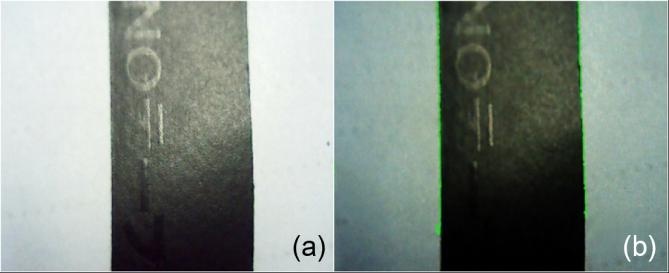
Fig. 11. Strong illumination scenario: (a) input image; (b) contour based on gamma corrected (γset ~ 0.5)
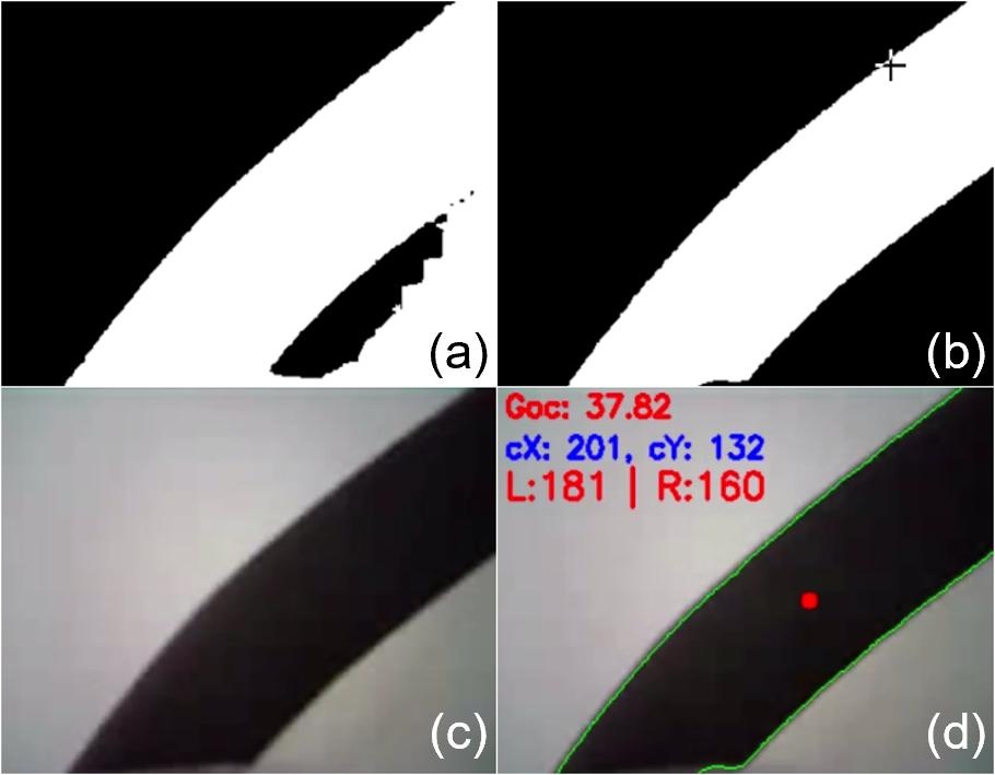
Conversely, in low light or shadowed scenarios (Fig. 12 and 13), the system sets the parameter γset to a higher level (2.4 and 2.8). The effective exponent γinv < 1 corresponds to the application of a logarithmic nonlinear transformation to amplify local contrast. Observations in Fig. 12a and 13a show that enhancement process successfully restored the blurred edge detail in the dark region.
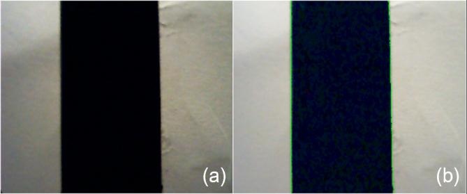
Fig. 12. Medium brightness scenario: (a) input image; (b) contour based on gamma corrected (γset ~ 2.4)
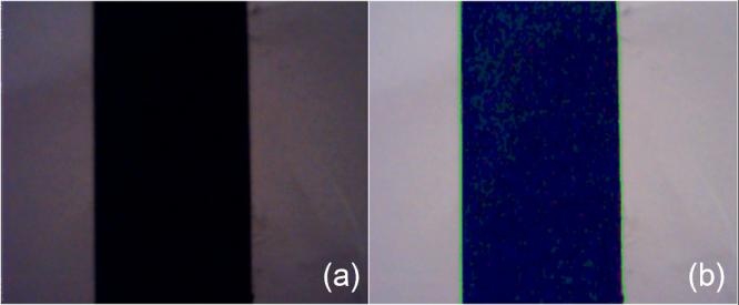
Overall, this continuous photometric normalization cycle significantly suppressed disturbances, stabilizing the input spatial characteristics. Therefore, the subsequent thresholding stage can accurately separate the main trajectory contours (Fig. 12b and 13b). This process provides a deterministic data foundation, ensuring high reliability for the loop steering control system.
Fuzzy control system response
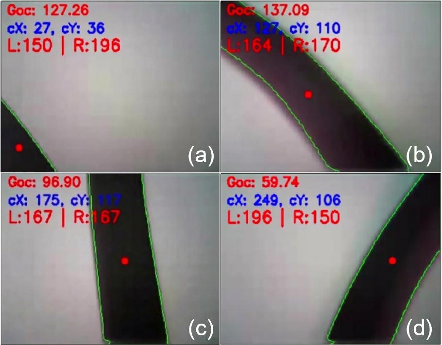
The effectiveness of the FLC was validated by monitoring the PWM outputs for the left and right motors in response to different θ and Cx. The experimental data for straight, right-turn, and left-turn scenarios are summarized in Tab. 2.
Tab. 2.
Experimental data for straight, right/left-turn scenarios
| Angle θ | Cx | PWML | PWMR | Behaviours |
|---|---|---|---|---|
| 37.82o | 201 | 181 | 160 | Fig. 14d |
| 127.26o | 27 | 150 | 196 | Fig. 15a |
| 137.09o | 127 | 164 | 170 | Fig. 15b |
| 96.90o | 175 | 167 | 167 | Fig. 15c |
| 59.74o | 249 | 196 | 150 | Fig. 15d |
As shown in Tab. 2 and visualized in: Fig. 15c, when θ was near orthogonal (80o - 100o) and the line centre was centred (157 < Cx < 177) the controller generated synchronized PWM signals (167/167) enabling stable straight-line motion; for right turns (Fig. 14d), the system detected θ < 90 ͦ combined with Cx ≥ 177, the controller immediately increased the left motor speed (PWML = 181) relative to the right motor (PWMR = 160) to execute the turn; and for left turns (Fig. 15a), the right motor speed was increased (PWMR = 196 and PWML = 150) to correct the trajectory.
The experimental results indicate that the dual input FLC supports line tracking by jointly exploiting θ and Cx. The deviation angle is treated as the primary cue for determining the steering direction, whereas the inclusion of Cx provides lateral-position feedback that contributes to loop stability.
As reflected by the rule outcomes for sharp right versus mild right cases in Tab. 1, different Cx linguistic regions lead to different PWM pairs even when the deviation is classified on the same side. In this manner, Cx is used to modulate the correction intensity to maintain the path centroid within the camera’s instantaneous field of view, thereby reducing the likelihood of sustained lateral drift.
Moreover, smoother transitions between straight and curved segments are promoted through the graded output levels and the Mamdani inference mechanism. In particular, rules associated with near-nominal conditions yield approximately balanced motor commands, which mitigates abrupt switching behaviour commonly observed in threshold-based line-following control.
However, the real-world execution of these control responses is inherently bounded by the system’s off-board processing latency. Experimental measurements indicate an average loop delay of ~350 ms, comprising image acquisition and Wi-fi transmission (~100 ms), PC-based image processing (~150 ms), fuzzy inference computation (~50 ms), and command feedback (~50 ms). While this phase lag has a negligible impact on straight-line tracking, it poses a risk of slight overshoots during sharp turns.
Dynamic response and tracking accuracy
The average loop latency of 350 ms, arising from communication overhead and Wi-Fi based off-board processing, necessitates restricting the system’s operational speed to 10-12 cm/s. At this velocity, the distance traversed by the robot during the command delay is approximately 3 cm. This displacement remains within the camera’s field of view, ensuring that the FLC maintains feature recognition and computes the necessary error compensation. Establishing this speed limit effectively mitigates overshoot and line tracking loss at curved segments and sharp turns. Experimental results confirm that the system maintains stable trajectory tracking without losing the guiding line at the operational speed of 12 cm/s.
The dynamic response of the tracking control system is analysed through the time varying PWM signals supplied to the left and right motors. Based on the experimental results illustrated in Fig. 16, the FLC demonstrates automatic modulation throughout continuous path tracking.
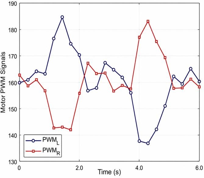
Specifically, between 1 s - 2 s, the trajectories exhibit a distinct separation: PWML increases sharply to approximately 185 while PWMR drops below 145. This interval represents a compensation phase for a sharp right turn, where the left wheel accelerates to redirect the robot toward the path centroid. Conversely, at approximately 4 s, a signal reversal occurs with PWMR reaching a peak of 183. This indicates sufficient system responsiveness to left hand curves or significant deviations in heading angle (θ) and lateral position (Cx).
Despite a loop latency of approximately 350 ms caused by WiFi transmission and off-board processing, the PWM curves maintain continuity without uncontrolled oscillations. Following each turning phase, the signals converge toward an equilibrium state (PWM ~160), resulting in stable motion during straight segments, notably between 2 - 4 s and 5 - 6 s. These results confirm that integrating heading information θ with lateral feedback Cx via the Mamdani inference mechanism ensures high tracking accuracy and significantly mitigates the abrupt switching behaviour typical of conventional threshold-based controller.
CONCLUSION AND FUTURE WORKS
This study successfully developed and validated a vision-based line-following robotic system robust to dynamic illumination variations. By synergistically integrating an automatic inverse gamma correction mechanism with Otsu’s thresholding, the system optimizes image contrast to ensure reliable path extraction under fluctuating light intensities, overcoming the limitations of static vision algorithms. The proposed multi-input Mamdani FLC, utilizing the relative deviation angle (θ) and horizontal centre coordinate (Cx), demonstrates stable trajectory tracking, effectively moderates mechanical oscillations and ensures smooth transitions between path segments and navigation scenarios at sharp turns.
The core contribution of this work lies in enabling the deployment of an intelligent control system on resource constrained hard-ware through an off-board processing architecture. Experimental results confirm that the system maintains reliable tracking and flexible responsiveness at an operational speed of 10-12 cm/s, effectively overcoming wireless communication latency challenges. While the current off-board setup introduces a loop latency of approximately 350 ms, the system remains feasible and suitable for intralogistics automation tasks in small and medium-sized factories.
Future research will focus on migrating the computational pipe-line to onboard edge computing platforms to minimize communication latency and increase robot movement speed. Additionally, optimizing the fuzzy inference rules via neuro fuzzy networks will be considered to further enhance the system’s dynamic responsiveness and operational efficiency. Furthermore, the integration of adaptive neuro-fuzzy inference systems will be investigated to automate the optimization of membership functions and rule bases, significantly improving the robot’s self-adaptability and tracking precision in dynamic environments.