
INTRODUCTION
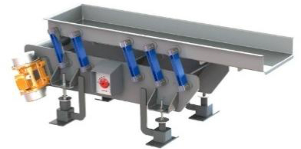
Antiresonant vibratory conveyors (Base – Excited Conveyors), shown in Fig.1, owe their rapidly increasing popularity to their two main advantages:
– Negligible, theoretically equal to zero, value of dynamic forces transferred to the ground during operation, resulting from the Frahm dynamic eliminator effect used in their construction, with the trough as the properly tuned eliminator mass [1], and
– Lower, compared to currently used over-resonant machines, required excitation force of vibrators, which induces vibrations of only a light transport trough, which does not require significant bending rigidity, as it is ensured by a massive body of the machine, and which is not burdened by significant masses of the drive system attached to this body.
Fig. 1.
VIBRAflex II Sanitary Antiresonant Vibratory Conveyor – PFI, which dynamic and discret model is presented in Fig. 2
These conveyors are becoming more and more widely used to transport loose materials [2], where dynamic forces transmitted to the ground by super-resonant conveyors are a significant disadvantage. For example, this is the case in mineral raw material processing plants, where flimsy buildings of processing stations, made of reinforced concrete, usually contain a considerable number of vibratory machines accumulated: conveyors, screens, dewatering centrifuges, etc., leading to intensive spread of floor vibrations, covering the majority of operation sites, endangering the health of operators and sometimes leading to building damage.
The antiresonance phenomenon is widely described in existing literature [3, 4]. Authors of [5] pointed out, that it is possible to determine the resonance frequencies of the structure under ideal boundary conditions, based on the experimentally determined antiresonance frequencies for structure under arbitrary boundary conditions. Renault et al. [6] proposed extension of linear concepts about antiresonances to the nonlinear cases of vibrating systems. The influence of transported material mass fluctuation has been analysed in [7], where authors presented nonlinear dynamic model of antiresonant vibrating machine.
The widespread use of antiresonant machines such as conveyors [8] or vibrating screens [9, 10] requires accurate and reliable methods of calculation, in which the correct determination of the antiresonant frequency and resonant frequency of the system plays a fundamental role. The development of anti-resonance vibration isolation methods is also important because more accurate computational models can be used both in the design of new systems and in the optimisation of the existing ones [11].
Due to the fact that there are a number of erroneous traditions in this field, usually resulting from misinterpretation, but also from the incompleteness of the dynamic elimination theory, this paper presents the basic mistakes made in this field, and the addition to Frahm’s theory and other phenomena to the extent required in the design of antiresonant machines.
THEORETICAL FOUNDATIONS OF ANTIRESONANT CONVEYOR OPERATION - DYNAMIC ELIMINATOR THEORY [12], [13]
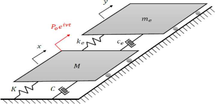
Antiresonant machines operate on the basis of the dynamic eliminator scheme [14], where the body of the machine, resiliently located and set in motion by a set of inertial vibrators, constitutes the protected object, while the transport trough, connected to the body by a set of springs, constitutes the mass of the eliminator. Let us denote the mass and the elastic and damping coefficients of the body spring elements by M, K, C, respectively, and the mass of the trough and the elastic and damping coefficients of the springs by me, ke, ce.
The operating principle of this system involves proper tuning of the eliminator [1]. The force in the eliminator spring (or spring system, in the case of a conveyor) reaches an amplitude and phase that counteracts the excitation force. For conveyors, this excitation force is the resultant force from the vibrators. When tuned correctly, the protected system (the machine body) nearly stops vibrating. This means it no longer transmits dynamic forces to the ground. Meanwhile, vibrations of the eliminator (the trough) enable the vibratory transport process.
Since this phenomenon occurs only in a narrow range of excitation frequencies [15] around the eliminator’s natural frequency (1)
(the so-called partial frequency, as it is not the vibration frequency of a combined system), wherein this frequency is closely surrounded by the resonant frequencies of the system on both sides. „The excitation and natural frequencies of the eliminator are subject to various interferences. Therefore, accurately determining these frequencies is essential for the machine's practical usability. These values significantly depend on precisely defined suspension parameters of the machine, including mass distribution, suspension stiffness and damping [1].Let us denote the absolute displacements of the masses M and me in the vibrations of the direction of the system by x and y, respectively, while the amplitude and frequency of the excitation force by Po and v (Fig. 2.)
Fig. 2.
Diagram of the dynamic vibration eliminator: M – protected mass, me – eliminator mass, K, C – constants of elasticity and damping of support elements of protected mass, ke, ce – constants of elasticity and damping of elastic elements of the eliminator, Poeivt – harmonic excitation force
The dynamic equations of motion of both masses are described by the following relationships:
The solution to the system of equations is predicted to be :
here A and B – vibrations amplitudes of the protected mass and the vibration eliminator and i – imaginary unitSubstituting the expected forms of the solutions of (3) into (2) resulted in the following relations:
4
Equations (4) can be represented in matrix form (5).
After solving the matrix system (5), absolute amplitudes of the form (6) and (7) were obtained for quasi-stationary values of v.
The partial frequency of the undamped vibrations of the protected system {M, K, C} is ωo (8)
and of the eliminator is ωn (9)(Since the frequency ωn (9) is at the same time an antiresonant frequency ωa, i.e., one at which body vibrations in the undamped system disappear, therefore, both designations are equivalent).
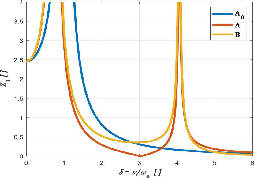
After assuming the coefficient values (Tab.1), an amplitude-phase diagram of the type shown in Fig. 3 can be obtained, on which the vibration amplitudes of the basic system without eliminator are usually plotted for comparison.
Fig. 3.
Plot of dimensionless amplitudes z1 for absolute displacements of the protected system A, the vibration eliminator B, and the system without the eliminator Ao, as a function of the ratio δ for the excitation frequency ν to the partial frequency of the eliminator ωn, equal to the antiresonant frequency (10) of the system, where z1 – the ratio of amplitudes to the value of static deflection of the protected mass
Tab. 1.
Parameters of the dynamic model from Fig. 2
| Parameter | Value | Unit |
|---|---|---|
| M | 600 | kg |
| me | 450 | kg |
| K | 719.387 | N/m |
| ke | 4.963.770 | N/m |
| C | 142 | Ns/m |
| ce | 298 | Ns/m |
| P | 14.450 | N |
As can be seen in Fig. 3, the vibration amplitude A of the protected mass M will be close to zero (red curve) at the antiresonant frequency (10).
This condition is a condition for dynamic elimination of vibrations by means of an additional attached mechanical system – the dynamic eliminator.
Graphs such as these are common in the literature and reproduce the position of the resonance frequencies for weakly damped systems quite faithfully, but they completely deform the vibration amplitudes, which results from the real excitation nature, depending on the square of the excitation frequency v. To make them more realistic, one can, for example, substitute the force amplitude Po in equations (6), (7) with the expression Po·(v/ωn)2. However, the route discussed below is much easier in order to determine the resonance frequencies of the system.
NOMOGRAMS FOR DETERMINATION OF RESONANCE FREQUENCIES
Around the resonance frequency (10) on its left and right sides there is an antiresonance zone, i.e. a region of frequencies for which vibrations of the protected mass M are the lowest. The values of amplitudes increase as one moves away from the antiresonant frequency, towards the resonance frequency forming a peculiar zone (Fig. 3. red graph). The width of the interval between the resonance frequencies is important for the safety of the system operation. The wider it is, the higher the operational safety, and therefore the more resistant the mechanical system is to various interferences of its operation. To precisely determine the safe operating range — which is not the subject of this study — it is necessary not only to determine the width of the antiresonant zone, but also to define the acceptable vibration amplitude limits, which requires a detailed analysis of each specific case and the corresponding identification of a safe operating frequency band. The primary objective for the designer of antiresonant machines should be to estimate the antiresonant frequency as accurately as possible and ensure that the system operates in its vicinity.
To determine the distance on the axis between the values of the natural frequency in a simple way, based on the solution of the damped linear system, we assumed ce = C ≈ 0. When equating the denominator of the expression (6) or (7) to zero with the damping neglected yields the expression (11), which allows to determine the resonant frequencies of the system, limiting the antiresonant zone:
Dividing the above equation by ke, K, and making further transformations and simplifications, we finally obtain the form (12).
To solve this equation efficiently, the assumption of equality of the partial frequencies of the eliminator and the protected mass (13) is used in the literature [12].
Using the notation (14) we obtain the final form of the foregoing equation for this case (15):
The roots of this equation are the following values:
The obtained dependence of the antiresonant zone width on the mass ratio only is shown in the graph in Fig. 4. The value of v/ωn = 1 for me / M = μ = 0 in Fig. 4 indicates that no eliminator mass was applied (me = 0). In this case, the resonant frequency is singular and determined solely by the main suspension. Attaching an eliminator mass on an additional suspension with a partial frequency equal to the partial frequency of the main suspension results in the emergence of two resonant frequencies, which appear on the graph on either side of the antiresonant frequency. This antiresonant frequency corresponds simultaneously to the partial frequency of the eliminator and the main mass. As a result, two curves are formed, representing the natural frequencies for a given μ value. When the eliminator mass increases, the mass ratio μ increases as well, leading to a greater separation between the antiresonant frequency and the two resonant frequencies. In case (13), the differences between the lower and upper resonances relative to the antiresonant frequency are practically identical.
Fig. 4.
Graph showing the ratio of the resonance frequencies to the antiresonance frequency v/ωn of the analysed system, compared to the ratio of masses me/M = μ in the equality of partial frequencies of the protected and eliminator masses
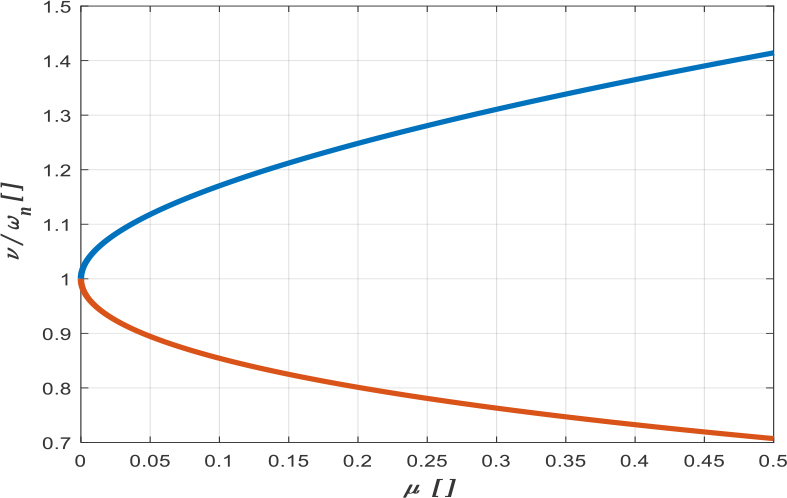
As can be seen in Fig. 4, the ratio of eliminator mass to main mass cannot be too low, as this reduces the antiresonant zone, and thus the system may be subjected to increased amplitudes when operating with a non-uniform load or other disturbances that may shift the operating point to a frequency close to the resonance frequency.
Unfortunately, this solution does not cover the case of antiresonant machines, since they do not satisfy the equality condition (13) of the partial frequencies of the object and the eliminator. Although a change in the support stiffness of the protected system K does not affect the existence and location of the antiresonant point, it does affect the location of the target natural frequencies of the main masseliminator system.) The aforementioned assumption (13) means only that a special case is considered when the protected mass is excited in its partial resonance. Having considered that, further conclusions based on this assumption would only apply to such a case, which obviously does not occur in soft-based antiresonant conveyor systems. This fact will be considered further on, where dependencies on the position of the resonance frequencies of the main mass – eliminator system will be derived, useful for analysing the operation of antiresonant conveyors.
EXTENSION OF THE METHOD FOR DETERMINING THE RESONANT FREQUENCIES PRESENTS THE CASE OF SYSTEMS IN WHICH THE MAIN MASS IS TUNED SUPER-RESONANTLY
To derive relations that define the location of resonance frequencies of the main mass–eliminator system in the general case involving the partial tuning of the main mass below the excitation force frequency, we will make the following additional assumption: we assume that the ratio of the antiresonance frequency (10) to the frequency of body oscillation on its spring suspension system (8) is represented by (17).
In this case, we get (18)
therefore (19) and (20)Inserting (18), (19), and (20) into (12), we obtain:
Transforming this expression by extracting the ratio v/ωn, we obtain the equation to determine the resonance frequencies at any tuning of the main system:
The roots of this equation are as follows.
Graphs showing the ratios of the upper and lower frequencies of the system to the antiresonance frequency ωa = ωn are shown in Fig. 5 for a typical operating range of antiresonant machines and, comparatively, for Δ = 1.
Fig. 5.
Graphs showing the ratio of the upper and lower resonance frequency to ωn as a function of the mass ratio μ, depending on the value of the parameter Δ. Note: upper frequency graphs for Δ>>1 values (Δ = 4 to 7) coincide approximately on the graph
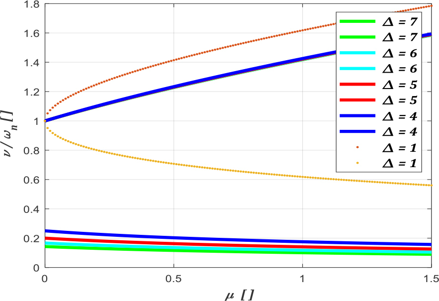
Comparison of the diagrams for Δ = 1 and those corresponding to typical super-resonant tunings of the protected system Δ = 4 to 7, leads to the conclusion that the nature of the two relations is different, wherein the super-resonant tuning of the main mass causes a downward shift of the resonant frequencies surrounding the antiresonant zone, causing a significant approximation of the upper resonant frequency to the operating frequency v = ωn, which increases the danger of accidental entry of the system into the nearresonant state.
To provide a better illustration of the effect of the parameter Δ (17) on the ratio of the resonance frequency to the antiresonance frequency, a graph, shown in Fig. 6, was prepared presenting four values of the parameter μ (14). These diagrams prove that for machines with bodies operating in the typical super-resonance regime, the main effect on widening the antiresonance zone is to increase the eliminator-to-body mass ratio, and for a fixed value of this ratio, it is advantageous to increase the parameter Δ, which, however, almost exclusively decreases the lower resonance frequency, leaving the upper resonance frequency, located relatively close to the excitation frequency, almost unchanged, much lower than the one resulting from the graphs for Δ = 1 (Fig. 4).

THE EFFECT OF THE ACTUAL NUMBER OF DEGREES OF FREEDOM IN A SYSTEM ON ITS CHARACTERISTIC FREQUENCIES
Although the theoretical analysis cited above allows the position of resonant frequencies to be determined with respect to the antiresonant frequency, which is the intended operating frequency of the system, this analysis does not take into account the fact that the actual system of an antiresonant conveyor has a much greater number of degrees of freedom, as shown in Fig. 5 on the example of a machine with a flat layout [16].
In particular, the actual system has the possibility and the specified frequency of the swinging motion α in the machine plane of symmetry, resulting in the actual lower limit of operating speed fluctuation possibly not corresponding to the lower resonant frequency of the eliminator considered earlier. These phenomena will be investigated during the modal analysis using the simulation model shown in Fig. 7.
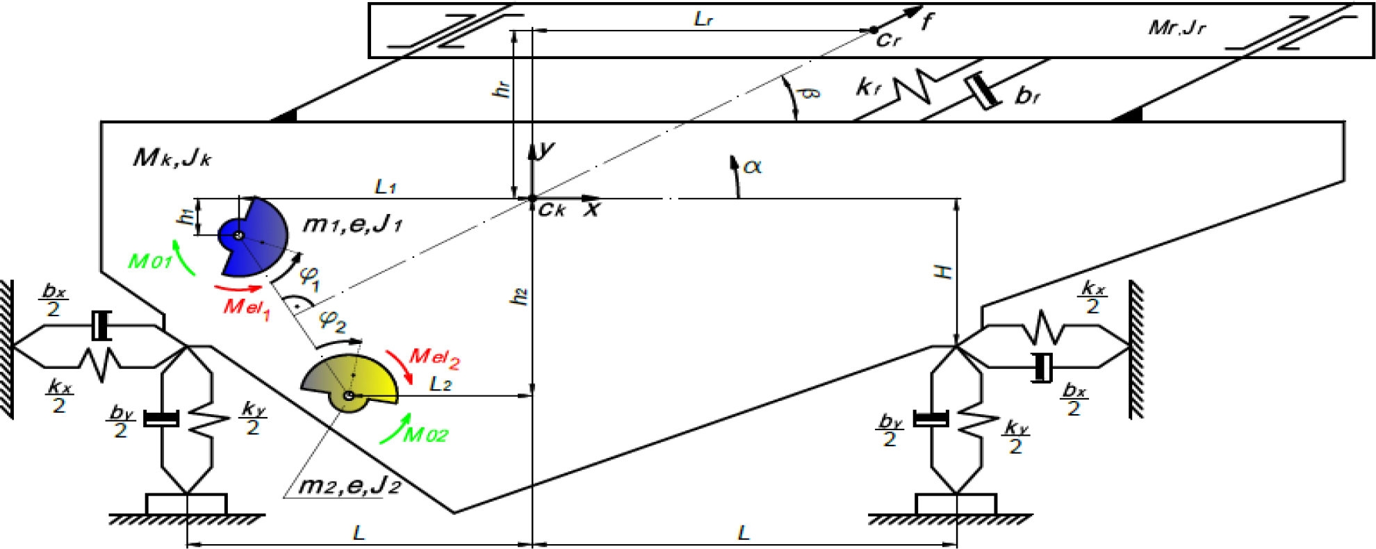
. Discrete dynamic model of an antiresonant conveyor
To perform a dynamic and modal analysis of the antiresonant conveyor, its discrete model formulated in [16] was used, with 6 degrees of freedom { x, y, α, f, φ1, φ2 }, as shown in Fig. 7. The model consists of two masses, i.e. the mass of the body Mk and the mass of the trough Mr, acting as a dynamic eliminator in this model, and two inertial vibrators with individual induction drive.
The body was spring-supported on helical springs fixed to the ground, while the conveyor trough was supported on spring rails fixed to the body. Counter-rotating inertial vibrators are the source of the resultant excitation force acting on the body at an angle β to the horizontal. The vibrators were mounted in such a way that the symmetrical segment connecting the centers of the vibrator bearings intersected the center of mass of the body and the trough. The following values of constants [SI] were assumed in the Tab. 2. and came from the literature [16].
Tab. 2.
Parameters of the dynamic model from Fig. 7
| Parameter | Value | Unit |
|---|---|---|
| Mr | 1000 | kg |
| Mk | 2500 | kg |
| Jk | 12200 | kgm2 |
| Jr | 5000 | kgm2 |
| ky | 2328000 | N/m |
| kx | 1164000 | N/m |
| kf | 10962000 | N/m |
| by | 0 * | Ns/m |
| bx | 0 * | Ns/m |
| bf | 0 * | Ns/m |
| L | 2 | m |
| Lr | 1.92 | m |
| H | 0.48 | m |
| hr | 1.1 | m |
| β | 30 | deg |
To analyse the motion of the system, in the static equilibrium state of the machine without a feed, an absolute central system was assumed in relation to the body of the machine, with the axes x, y, body rotation angle α, relative displacement of the trough relative to the body f and the absolute angles of rotation of the vibrators φ1 and φ2.
The set of equations describing the motion of the machine can be expressed in matrix form:
whereThe form of the mass matrix M and the vector of free expressions Q can be found in [2]. An approximate linearised form of these relations is used below to perform a modal analysis of the system.
. Linearisation of a Nonlinear System
Due to the low energy dissipation in the springs, mainly from material and structural damping, it is possible to analyse the natural vibrations of the system as undamped. The remaining nonlinearities of the machine model without feed are related to the effect of body vibrations on the vibrator motion and to the Coriolis acceleration in the compound motion of the trough. The dimension-to-mass ratios in typical vibratory machine designs generally allow the motion of the vibrator to be neglected in the natural vibration analysis and its mass to be focused on the rotation axis [12]. Similarly, when analysing the Coriolis acceleration value, it can be neglected compared to the other acceleration components for typical machine dimension ratios.
By doing so, the dynamic equation (24) can be reduced to the form (25)
in which: 0 – zero vector, M – mass matrix, K – elasticity matrix, where:Therefore, we obtain the matrix equation (27).
The existence of a non-zero solution to this equation is possible if the matrix(K – ω2 · M)is singular, i.e.
The relation (24) is a 4th degree equation on ω2 and leads to the determination of 4 natural frequencies (not necessarily different). We reject negative frequencies as physically meaningless.
After considering the form of the mass and elasticity matrices, we obtain:
whereAfter substituting the previously assumed numerical values and equating the determinant of the matrix (29) to zero, we obtain the following solution of equation (28) in the form of 4 natural frequencies:
. Forms of natural vibrations
Zeroing the principal matrix determinant means that the equations are linearly dependent, therefore it is not possible to obtain specific values of the amplitudes. By substituting a given natural frequency into the matrix, it is possible to determine the corresponding vibration form, that is, the ratio of amplitudes of individual coordinates. For specific values of vibration frequency, vibration forms were obtained in the form (30)
Calculation of the vibration form for a given natural frequency:
The form of the vibration related to the relative displacement amplitude f was obtained using the LU matrix decomposition.
For f1 = 2.61 Hz
Proceeding similarly for the other frequencies, the following was obtained in Tab. 3.
Tab. 3.
The form of the vibration
| f2 = 3.47 Hz | f3 = 4.41 Hz | f4 = 19.84 Hz | |
|---|---|---|---|
The form of the foregoing vibration forms indicates that the successive frequencies correspond approximately, respectively, to: horizontal vibrations of the entire machine, co-phase vibrations close to vibrations with lower frequency of the machine as an eliminator, angular vibrations of the machine and reciprocating vibrations of the trough and the body in the operating direction. The last form, which corresponds to the highest natural frequency, has the nature of an upper resonant frequency of the Frahm system.
If based on machine parameters we determine the value of the ratio of the trough mass to the body mass μ = 0.4 and based on the relations (23) derived for the Frahm’s model we calculate the value of the upper resonance frequency fu and the lower resonance frequency fl. Using formulas (10), (18), (23) and values from Tab. 2.:
where equivalent stiffness coefficient kxy is (34) and finalyWe obtain the following frequencies: fu = 19,83 Hz and fl = 3,32 Hz, respectively. The higher value is in satisfactory agreement with f4 of the machine, while the lower value reproduces f2 of the machine with an error of 4,3%. More importantly, the lower limit of the antiresonant zone does not correspond to fl, since the resonant region f3 of the machine, corresponding in the real machine to its angular vibration, is closer to the antiresonant frequency.
SPRING WEIGHT REDUCED TO TROUGH
In the case of antiresonant machines, the high stiffness of the spring system means that the mass of the springs is significant, accounting for about 1/4 of the trough mass, and should not be ignored when determining the antiresonant frequency. Since the spring is a deformable system, its mass "belonging" to the trough should be determined by determining the reduced mass. The lack of adequate values of reduction factors for springs in the literature makes it necessary to determine them.
To do so, assuming in line with reality that the first bending frequency of the spring positioned in its outermost points is many times higher than the operating frequency of the machine, to determine the deformation form f of the spring, we can assume that it is caused by the static application of force S in the operating direction – Fig. 8.
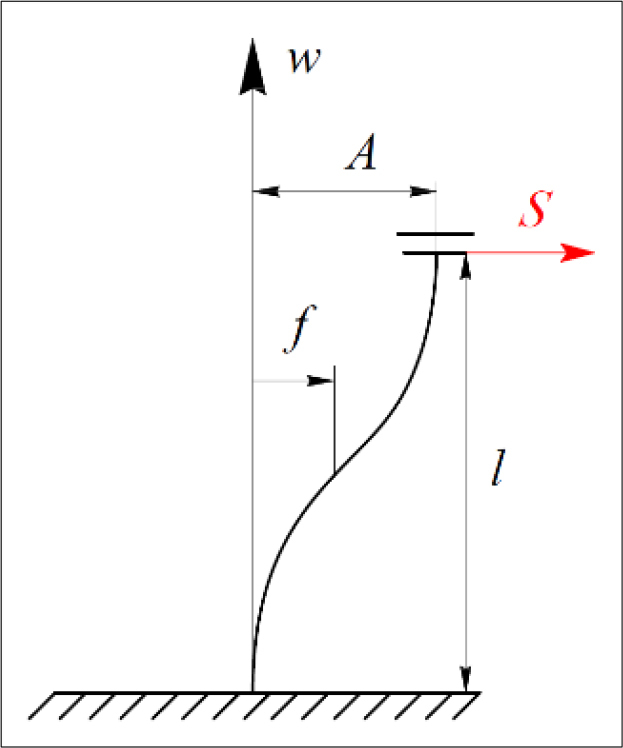
Let us denote by mj the mass of the active part of the spring. Taking advantage of the symmetry of the system, which leads to zero bending moment for w=l/2, let us write the equation of the deflection line of the lower half of the spring, i.e. for the range w=0 to l/2 in the form (36):
The solution to this equation (36) with boundary conditions (37) is (38)
Therefore, (39) were obtained.
where A=f(l) denotes the total amplitude of the relative displacement of both ends of the spring, equal to the vibration amplitude of the trough relative to the body in the direction f.By determining the S value from relation (39) and substituting it in equation (38) we obtain the deflection line of the lower half of the spring depending on A (40):
forUsing the antisymmetry of the deformation form of the upper and lower spring halves, the displacements of the upper part can be written in the form (41).
Between the time course of deflection f(t) and the speed course
Therefore, the square of the velocity amplitude of the point of the spring with deflection f is f2ω2. This allows us to present the maximum kinetic energy of the mass reduced to the trough as (42)
And the spring:
whereBy comparing the two expressions (42) and (43) for kinetic energy, the second of which is the sum of both parts of the spring, it is possible, after calculating the integral and dividing by A2ω2/2, to determine the reduced mass of the spring (45) which is connected with the trough and that produces the same inertial resistance at the attachment point as the tip of the spring.
Correct determination of the antiresonant frequency of the system requires adding the determined fraction of the mass of the active spring part to the mass of the trough (and, of course, the total mass of the grip parts associated with the trough).
. Experimental and numerical study of the frequency of bending vibrations
. An experimental model and Identification of system parameters and experimental determination of the first natural frequency
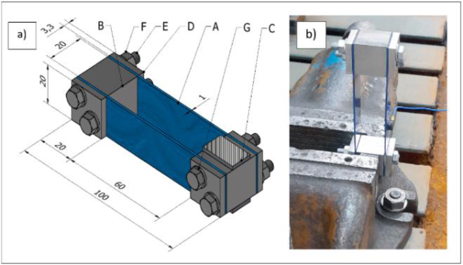
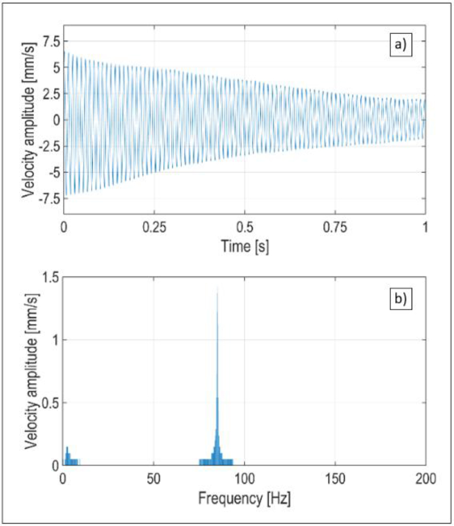
To check the accuracy of the calculation model taking into account the mass of the flat springs (Equation (45)), an experiment was carried out to determine the first natural frequency of bending vibrations of the system shown in Fig. 9. This system reflects the typical method of attaching flat springs in vibrating conveyors, such as the one shown in Fig. 1. attached by screws E, washers F and nuts G and pressure plates D to distancing bodies B. Figure 9a shows the basic dimensions of the elements of the analysed system. Figure 9b shows the system of Figure 9a attached by means of a vice to the anchored in the foundation. The vibrations of the free end of the system were induced by its deflection and release. Vibration recording was performed using a vibration analyzer KSD-400 from SENSOR equipped with a miniature accelerometer 352C22 from PCB PIEZOTRONICS with a mass of 0.5 g. The accelerometer was glued to one of the flat springs, as shown in Fig. 9b. The sampling frequency was 4.096 Hz. Due to analog integration, the vibration velocity was measured over time.
Fig. 9.
Scheme of the elastic support system, (a) A – flat spring, B – distancing mass, C – mounting washers in the vice jaws, D – pressure plates, E – screws M5x40, F – nuts, G – washers; (b) the system attached to the foundation with a vice
The results of free vibration tests of the system are shown in Fig.10. The time course of the vibration velocity decay is shown in Fig.10a. The results of the FFT analysis are presented on Fig. 10b. The natural frequency obtained from the experiments was 85,3 Hz.
In order to determine the actual elastic-inertial properties of the system, additional tests were carried out:
– three-point bending flexural tests of each of both flat springs, in order to determine their individual bending stiffnesses EJsi ;
– testing of the transverse stiffness kf of the entire system;
– measurement of the masses of system elements.
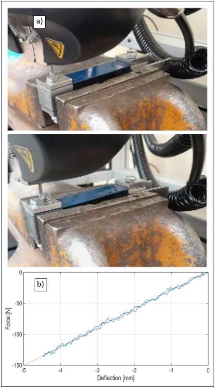
The values of the bending stiffness EJs1 and EJs2 of the used springs and the transverse stiffness kf of the entire system were experimentally tested using the MTS ACUMEN 3 testing machine, equipped with a 250 N force sensor. The traverse shift velocity in all tests was 0.5 mm/s. In the three-point bending flexural tests, the distance between the supports was 70 mm. Figure 11 shows a stand for three-point bending flexural tests and a graph of the lateral force versus the deflection arrow for one of the springs, along with a 1st degree polynomial approximating this course. Approximations of the experimental results were performed in the MATLAB software environment. The values of the slope coefficients of the linear approximating functions were 48.7078 N/mm and 48.4407 N/mm respectively, while the coefficients of determination were 0.9991 R-squared and 0.9992 R-squared respectively. Based on these values and the known relations, the bending stiffness values of the two springs were determined, which were EJs1 = 348058 Nmm2 and EJs2 = 346149 Nmm2 respectively. Figure 12 shows the entire system subjected to transverse load (Fig. 12a) and the relationship between transverse force and stiffness kf of the system along with a function that approximates stiffness (Fig. 12b). The approximate stiffness value was 30.4068 N/mm, with a coefficient of determination of 0.9967.
Fig. 11.
An experimental determination of the transverse stiffness of flat springs: (a) view of the station, (b) force-displacement diagram for one of the spring
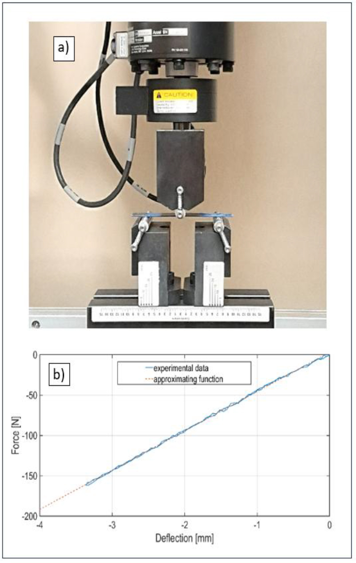
Fig. 12.
Experimental determination of the stiffness of the entire system (a) before and after the load, (b) the relationship between the transverse force and the stiffness kf of the system
The information contained in Tab. 4 with the following notations was obtained from the analysis.
Tab. 4.
Geometric and physical parameters of flat springs and other components of the test system (Fig. 9) - mass values are given with an accuracy of 0.01 g
. The 1st natural frequency – a continuous and discrete model
The impulse excitation was used to perform a modal analysis, i.e. the appearance of a short-term high force acting across the springs. The appearance of this force causes the excitation of resonance vibrations. These vibrations also include the first form of natural vibrations, which is related to the deformation of the springs of mass mr and the oscillations of the mass md, which is the sum of the masses of the non-deformable parts (distancing mass (B), screws and washers (E)). The behaviour of the vibrating system with the first mode of natural vibrations from Fig. 9 shows not only the continuous model (Fig. 13a), but also the discrete model (Fig. 13b), which simplifies the behaviour of the system for the translational movement of the mass mz (due to the identical displacement of the mounting points of the flat springs). The mass mz is the reduced mass of the vibrating elements, i.e. masses of the deformed springs mr and the nondeformable vibrating parts md. Using formula (45), the reduced mass mz was obtained in the form (46).
Fig. 13.
Continuous model of the tested system showing the first natural frequency (a), discrete equivalent model of the tested system for the first natural frequency (b)
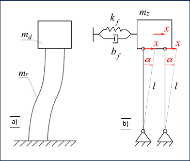
In this case, the replacement suspension system was a spring and damper package with stiffness and damping coefficients kf and bf, respectively, attached to the support and the reduced mass mz parallel to the direction of vibration.
The elasticity of a single flat spring used in the experiment was calculated from the Eq. (47), which takes into account the constant moment of inertia (48) of the cross-section b x h of the spring bar shown in Fig. 9a and Tab. 4.
whereThe energy absorption coefficient ψ for flat steel springs is equal to 0.04 [17], which means that the viscous damping coefficient of the spring is so small that its impact on the vibration frequency is negligible. After taking into account the parallel connection of flat springs and the discrete model, the doubled elasticity kf and the first natural frequency of undamped vibrations (doubled damping coefficient bf ≈ 0) in the form (49) were obtained.
Frequency not taking into account the spring mass calculated from the Eq. (50)
. The 1st natural frequency – a numerical model
FEM software is usually used as a tool to check the accuracy of analytical calculations carried out in the conveyor design process. Modal analyses are most often used to determine the natural frequency of the system. The results of such an analysis, performed in the ANSYS software environment, are presented below. The inertial and elastic parameters of the solid model were determined on the basis of experimental data presented in Tab. 4. Due to differences in the geometry of the real elements and the solid model (e.g. modelling the threaded part of the screws in the form of a cylinder, omitting chamfers, etc.), appropriate density values were assigned to individual elements in the solid model so that their masses were consistent with those measured experimentally. The Poisson number for all elements was assumed to be 0.3, and the Young's modulus of springs was assumed to be 208262.1 MPa, which is the average of the values determined on the basis of experiments. For the remaining elements, a value of Young's modulus representative for carbon steels was assumed, equal to 200000 MPa. In order to obtain a high-quality FE mesh, the selected elements were divided into smaller volumes and then the requirement for compliance of common nodes was imposed within these elements. All parts of the system have been discretised using higher-order finite elements exhibiting quadratic displacement behavior. Springs have been discretised using quadratic 20-node hexahedral elements, which generally give more accurate results than tetrahedral-shaped elements and are also more reliable in terms of the skewness parameter [18, 19]. To obtain reliable results from the FEM analyses, in addition to analysing the quality of the FE mesh, an additional analysis of the influence of the density of the spring modelling mesh was performed. Modal analyses were performed with three finite element mesh settings in the spring thickness direction b: with one, two, and three finite element layers. The models obtained in this way are shown in Fig. 14. In Figure 14, the boundary condition of the restraint on the surface of the mounting plate on the FEM model is additionally marked in yellow. Table 4 lists the number of nodes in individual system models, the results of the FE mesh quality analysis (average skewness and average orthogonal quality), and the results of the impact of the FE mesh density on the natural frequency value obtained in the modal analysis.
Fig. 14.
The results of the modal analysis performed in the ANSYS environment - the first form of vibration from Fig. 8 and 9 - the simulation result is 97,74 Hz (Tab.4) for three finite element layers on flat springs

The difference between the results (Tab. 5.) obtained for models with 3 and 2 layers was approximately 0.06%, indicating the high accuracy of the results. These results are in good agreement with the result of the formula (49) taking into account the mass of the spring (97.33 Hz). The difference between the pattern result and the 3-layer FEM result was approximately 0.4%.
Tab. 5.
Parameters of modal analysis
. Comparison of analysis results
In the comparative analysis, the reference value with which the remaining results were compared is the frequency of the first form of vibration obtained from the experimental analysis, which was 85.3 Hz. As shown in Table 6, the result of the theoretical analysis of 97.33 Hz, taking into account the reduced mass of flat springs (49), is closest to the value obtained from the experimental test. The difference in values and the relative error of 14.10% may result from assembly errors and measurement errors when determining the active length of the flat spring.
Tab. 6.
Comparison of the frequency results of the first form of bending vibrations
| A type of modal analysis | f [Hz] | ε[%] * |
|---|---|---|
| theoretical without taking into account the mass of flat springs | 100.83 | 18.21 |
| theoretical taking into account the mass of flat springs | 97.33 | 14.10 |
| numerical | 97.74 | 14.58 |
| experimental | 85.30 | 0 |
The active length should be counted from the place where the spring is attached, taking into account the chamfers of the spacer mass (B) and the pressing washers (D) from Fig. 9. The theoretical method does not take into account their deformability, which could occur under real conditions. Failure to take into account the mass of the springs (50) with the result of 100.83 Hz leads to even greater errors in frequency estimation at the level of 18.21%. The numerical analysis gave a result very close to the theoretical value, taking into account the reduced spring mass. Both of these methods assume tight adhesion of the springs and spacer masses to each other, and hence the active length in both methods is identical. In fact, due to the slight deformability of the handles, the active length can be greater and the elasticity of the springs can decrease with the cube of the active length of the spring (45).
CONCLUSIONS
Achieving high mobility properties of conveyors operating on the basis of Frahm's principle of dynamic elimination requires high accuracy in determining both the position of the antiresonant point and the resonance frequency of the system. Relationships based on the classical Frahm damping theory lead to results that are far from real in this regard. This paper presents correct derived formulas and a nomogram built for designers based on them. The effect was shown that the actual number of degrees of freedom in machines constructed using the dynamic eliminator principle has on frequencies limiting the antiresonance zone. The effect of the spring mass on the antiresonance frequency was also pointed out, and correct relations for its consideration were derived. The issues discussed do not exhaust the possible causes of unsatisfactory running properties of antiresonance type conveyors. Many significant errors may also result from a simplified mathematical description of the vibrating system, not including the phenomenon of self-synchronisation of vibrators [7] or even the construction of a system that does not guarantee the possibility of obtaining the exciting force along a straight line [20], which is the cause of the component of the direct transfer of the exciting force to the ground.