
INTRODUCTION
Helical compression springs are widely used in mechanical engineering. The primary functions of springs are absorbing energy and mitigating shocks, applying a definite force or torque, supporting moving masses, isolating vibrations, indicating or controlling load or torque and providing an elastic pivot or guide [1]. Consequently, they find widespread application in vehicle suspensions, such as those in cars [2], railway bogies [3, 4], vibratory conveyors [5], internal combustion engine valves [6], and vibration absorbers [7]. Springs operate under static and dynamic conditions and are subject to buckling. In specialized applications, these performance characteristics must be determined with high precision. This necessitates precise design, including a meticulously shaped coil configuration. In the paper [8] a method for modeling helical irregular polymer structures and determining their stiffness and stresses in a numerical and experimental way is presented, showing the possibilities of numerical methods in geometry modeling. Most designers still rely on basic helical structures, which have not been thoroughly studied. One aspect of spring construction that remains insufficiently studied is the end coil, whose shape influences the spring's stiffness and the distribution of transverse forces resulting from axial compression [9]. However, the precise extent to which the shape of the end coil influences the spring's stiffness, and the distribution of transverse forces has not yet been thoroughly evaluated. The motivation for conducting research in this area arises from the occurrence of spring failure [10, 11, 12], especially damage in the form of coil fractures near the inactive coil [13, 14]. In paper [10], using FEM analysis of an automotive barrel spring, the stress distribution of on its surface was investigated in the area around a modelled failure in the form of a blind hole. In paper [11], a numerical analysis of a torsion spring made of round wire was carried out, indicating the locations of possible fatigue cracks initiated by defects created by machining. This is also related to both axial and transverse stiffness, which significantly affects load transmission [15, 16], and is directly linked to the transverse forces generated by compression [17].
The inaccuracy in determining the stiffness of a spring arises from at least four factors, which include dimensional inaccuracies in the geometric parameters of the spring, such as the wire diameter d, the mean coil diameter D, the number of active coils na (which decreases during compression), and errors in estimating the modulus of rigidity G [18]. Additionally, a smaller influence on the spring's characteristics is attributed to the helix angle γ, which can be neglected for springs with angles smaller than 10 degrees, or even 15 degrees (resulting in an error of only 2.5%) [1]. Wahl indicates that the parameters mentioned earlier, as well as the shape of the end coil, have a greater influence on stiffness than the helix angle. Therefore, deviations in the helix angle along the entire length of the spring have an even smaller effect. The paper [12] also highlights the problem of non-uniformity of pitch and wire diameter, but also hardness, which affect the stiffness characteristics of the spring. Further factors mentioned in the literature include errors in the perpendicularity of the spring axis to the support surfaces [18], the type of end coil used [19], and the transition between inactive and active coils associated with it [20]. The latter factor can significantly contribute to nonlinearities, especially if the progressive transition zone is large [21]. The way the spring is assembled also affects its characteristics, i.e., whether the spring ends are fixed or free to rotate [1], which also leads to variations in the detailed formulas for axial stiffness [18]. The continuous change in structural parameters D, na, and γ during spring deformation results in the development of nonlinearities in the spring's characteristics [18]. During compression, nonlinearity initially arises from factors such as the non-parallelism of the spring ends, the lack of perpendicularity between the spring axis and the support surfaces, load eccentricity, and errors in the contact of the inactive coils. In the final stage, nonlinearity is caused by the non-simultaneous blocking of active coils. For this reason, it is recommended to calculate the axial stiffness within the central range of the spring’s characteristics, i.e., for forces within 0.3 to 0.7 of the spring’s blocking force Fn [18]. Additionally, the process of loading and unloading a compressed spring exhibits hysteresis [22], which means that stiffness may not necessarily have the same value in both loading directions.
Differences in the value of axial stiffness also result from the development of transverse forces during compression. In [9], the causes of transverse forces were presented, including spring asymmetry, load misalignment, buckling, stresses, variable wire diameter, and pitch variation. When these factors are significant, larger transverse forces are generated, which reduce the axial force and, consequently, the axial stiffness of the spring. The highest transverse forces occur in conical springs [9]. The issue of axial force transfer is addressed by recommending the use of a fractional total number of coils. In this configuration, the ground ends of the spring are arranged in opposite directions, preventing load misalignment [18]. Springs typically have one inactive coil on each end, but for long springs and under variable loads, 2 or 2.5 inactive coils are used to improve spring stability [18, 23]. Conventionally, the boundary between active and inactive coils is considered to be the point where coil contact begins in the unloaded state. However, this point is movable during compression, and it has been shown that part of the inactive coils primarily experiences torsional stresses [24]. For this reason, it cannot be assumed that the entire inactive coil does not contribute to the spring's stiffness. The EN 13906-2013 (E) standard [25] does not acknowledge this fact, adhering to the conventional boundary principle. This applies to supported coils, as defined in the ISO 2162-2:1993(E) standard [26]. For springs with open-ground ends, the inactive coil begins at the start of the ground surface, whereas open-unground springs lack an inactive coil. Such springs require specialized mounts using, for example, elastomer inserts [27]. In such cases, the boundary between inactive and active coils may be where the spring exits the fixture, although this depends on the degrees of freedom provided by the fixture. Transitional coils, which lie between inactive and active coils, are also identified [20]. This distinction arises from a pitch difference compared to the active section, which increases nonlinearly. It has been shown that the length of the transitional coil influences the magnitude of transverse forces and, consequently, axial stiffness [20]. The lack of standardized methods for defining the boundary between spring coils causes discrepancies in measurement results compared to the basic formula for the spring rate k provided in EN 13906-2013 (E) [21]. The full formula, which accounts for the helix angle, is not widely used, as helix angles typically do not exceed 10°, and spring indices greater than 10° result in minimal calculation errors [28]. One way to improve formula accuracy is by adding a correction factor to the number of active coils. The first proposal was made by Vogt [29], who suggested adding 0.5 to the number of active coils. Later, Paredes [30] proposed a correction of 0.35 and introduced a version that adjusts both the number of coils and the spring height, achieving an error of less than 0.2 compared to experimental force measurements. Additionally, Paredes demonstrated that the relationship in EN 13906-2013 (E) provides sufficient accuracy for springs with more than five active coils. In [28], formulas were developed to calculate the axial deflection of springs with rectangular, square, circular, annular, and elliptical wire crosssections. The study analyzed stress contributions from axial force, shear force, bending, and torsional moments. It also presented formulas proposed by Wahl, Timoshenko, Ancker, and Goodier. The results were compared with finite element analyses performed in ANSYS, showing that the Ancker and Goodier analytical formula yielded the most accurate results. The formulas by Yıldırım and Timoshenko take the helix angle into account [31]. A similar assumption is made in the Krużelecki and Życzkowski formula [32], which provides results comparable to those of Timoshenko. In [33], Hiroyuki's formula was introduced, which incorporates material constants E and G, as well as the tangent of the helix angle. In [31], a more accurate formula than those of Timoshenko and Hiroyuki was proposed, though it is highly complex, incorporating parameters such as wire inclination K, spring wire length L0, and Poisson's ratio ν. Liu and Kim [24] proposed adding spiral ends to the active coils of helical springs, modeling the torsional stresses occurring in the end coil. They supported their findings with finite element simulations. Using Castigliano's theorem, they derived a correction factor for the end coil, which should be multiplied by the classical formula to account for its effects.
The aim of the study is to determine the effect of varying the contact length between coils on the axial stiffness and transverse force resulting from the axial compression of springs with ground and supported end coils, as specified in ISO 2162-2: 1993 (E) [26]. The research will be conducted using a tensile testing machine and numerical methods. Additionally, the results for axial stiffness will be compared with commonly used formulas, and empirical equations will be proposed to predict the axial stiffness and transverse reaction forces. This study's main novelty lies in its comprehensive quantification of how end-coil geometry significantly affects not only axial stiffness but also the magnitude and direction of transverse reaction forces — areas previously lacking precise analytical relationships in the literature. From an industrial standpoint, the new relationships enable more reliable spring design, particularly in suspension systems, vibration absorbers, and conveyor mechanisms — applications where unaccounted transverse reactions can lead to misalignment, fatigue fracture, or operational instability. Ultimately, the improved predictive accuracy supports enhanced performance, safety, and longevity of springs in automotive, rail, and industrial machinery contexts, enabling engineers to design with tighter tolerances and fewer prototypes.
ANALYTICAL METHODS
In the literature, several formulas for determining axial stiffness are distinguished, some of which were mentioned in the introduction. The most commonly used formula for the axial stiffness kN is the equation (1) provided in the EN 13906-2013 (E) standard [25], which does not take the helix angle γ into account.
where G represents the modulus of rigidity, d is the nominal diameter of wire, D is the mean diameter of coil, na represents the number of active coils.Among the methods that increase the accuracy of axial stiffness calculations for springs, the most popular and straightforward ones were selected, which, after preliminary analysis, yield results that differ from each other.
As mentioned in the introduction, Vogt [29], in order to account for the influence of the inactive coils, proposed increasing the number of active coils by 0.5. On the other hand, Paredes [30] verified this and introduced an increase of 0.35 in the number of active coils. This value is named as correcting number of active coils ncor, which is used in formula (2), describing Vogt (V) or Paredes (P) method.
A more accurate method compared to equation (1), which takes the helix angle γ into account, is the formula (3) proposed by Krużelecki and Życzkowski [32], which slightly changes the value of the axial stiffness compared to equation (1).
where Ct0 represents the initial compression stiffness, R0 is the initial spring radius, ν represents Poisson's ratio, E is the Young modulus, I represents axial moment of inertia of spring wire, γ represents helix angle and Ha is the height of unloaded active coils.In the publication [28] Yıldırım proposed equation (4), which takes into account the shear stiffness Cb, compression stiffness Ct, bending stiffness Db and torsion stiffness Dt, expressed by equations (5–8), respectively.
Another method accounting for the inactive coils was presented by Liu and Kim in their publication [24], where they introduced the concept of end coils above the ground surface. The number of these coils should be added to the active coils and placed in the denominator of the ratio, with the numerator being the number of active coils. This is represented by equation (9).
where xn is the number of coils from the bottom to a certain point of the spring and xend is the number of effective coils at the bottom [19].The presented formulas will be compared during the numerical analysis stage, aiming to find the smallest mean absolute percentage error (MAPE) in order to identify the methods that provide results closest to reality and to propose a new method.
MECHANICAL TESTS
. Stiffness experimental tests settings
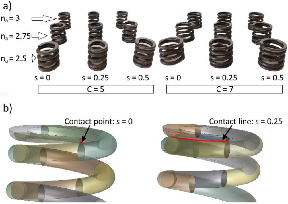
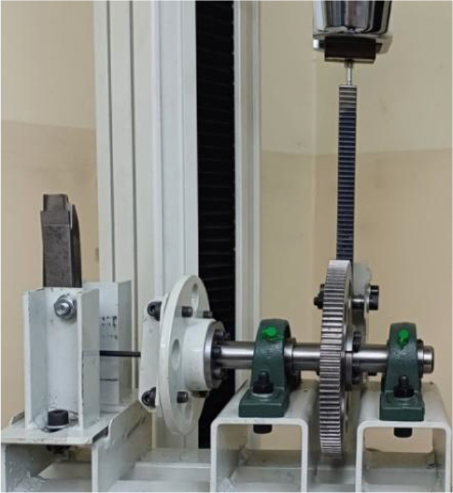
The spring compression tests were carried out using an HT-2402 testing machine from Hung Ta Instrument Co., Ltd., Taiwan, equipped with a CL16md 5kN load cell from ZEPWN, Poland, of the precision class 0.5 according to ISO 376 (Fig. 1) [15]. The results were recorded using dedicated software. The test sample consisted of 18 sets of springs with squared and ground end-coils, each containing 3 identical springs in terms of their parameters. In total, this amounted to 54 springs. The spring sets (Fig. 2) differed in the spring index C, which was 5 or 7, the number of active coils na, which was 2.5, 2.75, or 3, and the contact length of the end coils s, which was 0 (point contact), 0.25, or 0.5. The contact length s was defined as the quotient of the length of the contact line between the end coils on one side of the spring and the length of one coil of wire. It was determined by inserting a 0.07 mm thick plate of feeler gauge until it locked in place. Then, using a protractor with a resolution of 1 degree, the angle of the arc from the end of the spring to the locking point of the slotted gauge plate was measured. The pitch P of the springs equaled 10 mm for all springs.
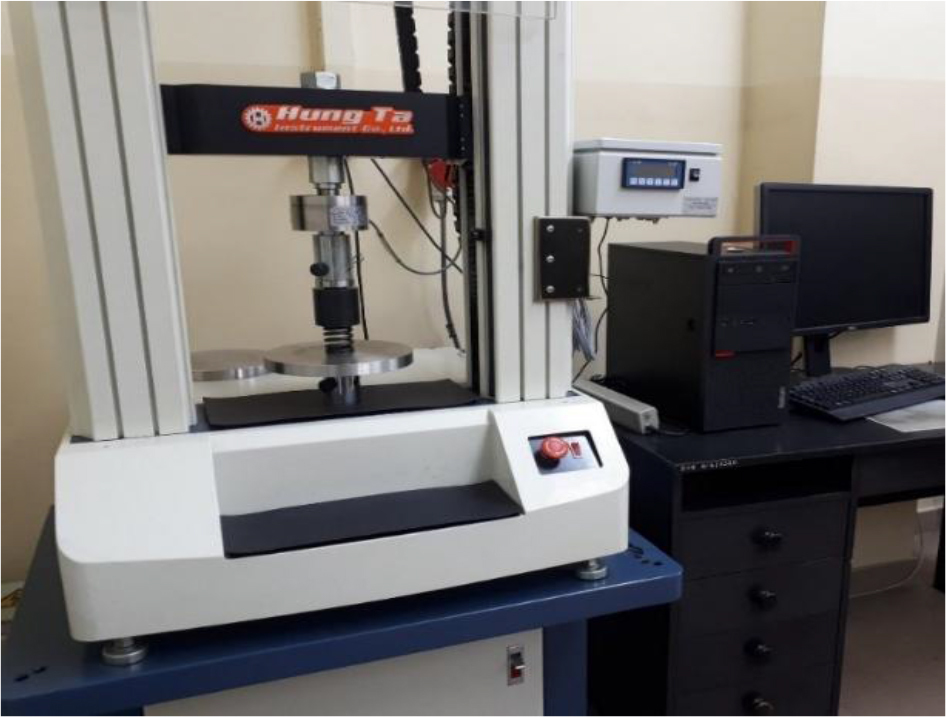
Fig. 2.
Samples of springs (a) used to axial stiffness researches; (b) graphical representation of contact length for two example lengths s = 0 and s = 0.25
The springs were supplied by a company specializing in custom-made springs. They were manufactured in accordance with the EN 13906-1:2013 standard [25]. The springs were made from 55CrSi FD Becrosi 26 spring steel, which complies with the EN-10270-2 standard [25]. The wire diameter d was nominally 5 mm with upper and lower deviations equal to respectively: +0.008 mm and -0.010 mm. The main material properties of this steel include a modulus of elasticity in tension E of 206 GPa, a modulus of elasticity in shear G of 79.5 GPa, and an ultimate tensile strength Rm of 1800 MPa. The first technological process involved coiling the springs. Next, the springs were tempered at 220°C for 15 minutes, after which the end coils were ground to ¾ of the circumference. Finally, the same heat treatment was applied again [15].
The springs were measured in terms of height using an elec tronic caliper and the number of coils in contact using a protracto with an accuracy of 1 degree. The reference point was the theoret ical height, calculated as the product of the pitch P and the numbe of coils n, while for the contacts, the measurement corresponded to the order specifications. The springs that were closest to the bench mark geometry were considered as reference specimens for vali dating the numerical model. These were precisely replicated, and their measured axial stiffness became the benchmark for calculat ing the accuracy of the numerical model. The axial stiffness k in the bench tests was calculated according to Eq. (10). The maximum deflection for each spring was half of the theoretical spring gap, and the minimum reading point was 20% of the maximum deflection Therefore, the maximum deflections for the springs with 2.5, 2.75, and 3 coils were 6.25 mm, 6.875 mm and 7.5 mm, respectively.
where Fmax, Fmin – force, Smax, Smin – deflections for the maximum and minimum measuring point, respectively.. Results and initial analyses
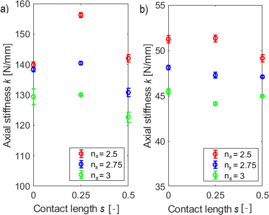
The results of the axial stiffness tests are presented in the form of a scatter plot (Fig. 3), with error bars indicating the variability range of the 3 measured samples. The variability was minimal, indicating repeatability of the results. When comparing the springs in terms of contact size, an increase in axial stiffness was observed for the 0.25 coil contact, which requires further investigation. These changes are particularly significant for the shortest spring with a spring index C = 5, where the ratio of the data spread to the mean was equal 11.2%. For the same number of coils but with a spring index C = 7, this ratio was 4.3%. A higher spring index also results in greater stiffness for point or quarter-coil contacts, although this effect is less apparent than for the springs with smaller index. It was decided to extend studies with a numerical model to highlight specific trends in the changes.
NUMERICAL TESTS
. Material research
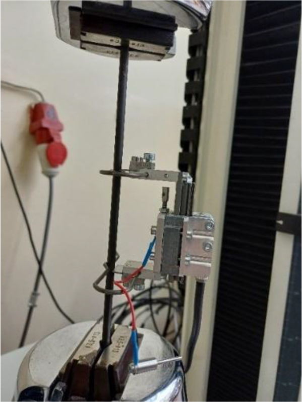
To build a more accurate numerical model, measurements of Young’s modulus E, Kirchhoff’s modulus G, and the coefficient of friction for the material from which the spring wire was made were performed. The measurement of Young’s modulus E was conducted for two samples of straight wire with a diameter of 5 mm, sourced from the same spring manufacturer. The tests were carried out on the same testing machine equipped with load cell CL16md 5kN and a ZEPWN CL 25D-R B50 L30 extensometer, with resolution of 1 μm (Fig. 4). Tension was carried out under crosshead control at a speed of 1 mm/min, with the length of the entire specimen between the grips being approximately 180 mm. As a result of the measurement, elongations and stresses in the wire cross-section were obtained, as shown in Table 1.
Tab. 1.
Results of Young’s Modulus E measurement
Young's modulus was calculated according to the relationship given in ASTM E111 – 04, based on the values given in Tab.1. The increase in force divided by the original cross-section of the specimen corresponds to the difference in stress σ2 and σ1, while the increase in strain corresponds to the quotient of the difference in elongation L2 and L1 and the original measurement length L0. Averaged over the two measurements, the value of Young’s modulus was 204031 MPa.
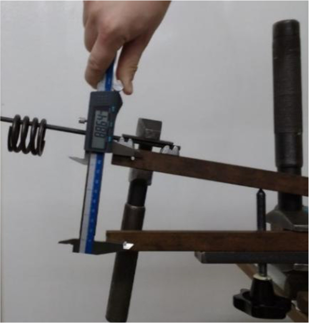
The next stage involved measuring the shear modulus G. The measurement was conducted using the same testing machine, but with an extension for twisting rods (Fig. 5). To secure the rod in the extension, it was bent, leaving a section L equal to 112 mm. To avoid damaging the samples, the measurement was repeated 14 times on the same rod, with the traverse displacement of the testing machine set to 20 mm. The first 3 results were excluded due to significant deviation, and the average force was calculated to be 118.6 N, with a coefficient of variation of 0.6%. The calculations based on formula (11), resulted in a shear modulus G value of 80,550 MPa.
where: F – force measured by the sensor of the testing machine, Rg – radius of the gear wheel of the attachment, L – twisted wire length, φ – wire twist angle obtained by measuring the axial displacement of the testing machine crosshead, d – wire diameter.
The final key material property is the coefficient of friction μ. Two coefficients were distinguished - one larger for the ground surface in contact with the machine supports and a smaller one for the contact between the wires. The friction coefficient between the contacting wires was measured using a constructed bench based on an inclined plane (Fig. 6). There is currently no international standard that specifically addresses the measurement of the coefficient of friction between round steel bars. A straight spring wire was fixed, and the shortest spring was placed on it, with the measurement repeated 6 times for 3 samples of the same spring on two inner sides of the springs, giving 36 results. This way, point contact was achieved between 4 coils and the wire. The flat surface was raised until the spring began to slide. As a result of the data analysis, 6 values significantly deviating from the average were discarded, resulting in 30 values, which were used to calculate the average coefficient of friction. The range of variation of the friction angle spread from 0.153 to 0.186.
Using geometric relations, the friction coefficient was calculated as the tangent of the friction angle. Average value of measured friction coefficient was equal to approximately 0.18. The result was considered to be determined with sufficient accuracy, also confirmed by literature [34]. This parameter also depends on pressure force [34]. For the ground surfaces, it was assumed that the friction coefficient would be much higher than for smooth surfaces, and in the numerical analyses, it was taken as 0.5. This value is also one of possible for steel to steel pair [34] and steel to aluminium pair [35]. Under actual operating conditions of helical compression springs, the friction forces between the spring's ends and the supports should be greater than the transverse reaction forces. Otherwise, there would be abrasion of the ground wire surface, which would increase the risk of wire fracture and could also result in a loss of support stability. If it is anticipated that the transverse forces may be greater than the frictional forces, then the support of such a spring is strengthened by shaped end protection, e.g. in the form of pins or cylinders centering the spring end coils. Such solutions are used, for example, in vibrating machinery and in railway bogies. Therefore, the adopted value for the friction coefficient, ensuring no slippage between the analysed spring models and their supports, ensured at the same time a correct representation of the actual working conditions of this type of spring.
. Numerical model
The numerical simulations were performed based on the finite element method using Ansys Workbench software, specifically the SpaceClaim, Design Modeler, and Static Structural modules. Each model was created using a script described in the publication [21]. By transforming the formulas presented there, the radius of the arc aligning the pitch between the applied and active coils was calculated in Matlab. By inserting this radius, the spring helix angle γ, spring index C, and wire diameter d into the program’s algorithm, a code was generated that could be input into SpaceClaim. In this software, the spring ends were cut to ¾ of the circumference. Then, in the Design Modeler module, the spring was splitted along its axial planes, dividing each coil into four equal parts and creating the contact surfaces needed for the next stage of model construction. Two supports in the form of rings, with a thickness of 0.2d and diameters slightly different from the inner and outer diameters of the spring, were also added. An example of a spring modeled in Design Modeler is shown in Figure 7a.
Fig. 7.
Spring with parameters C = 5, d = 5 mm, na = 2.5, s = 0.25 with supports a) modeled in the Design Modeler module of Ansys Workbench software, b) mesh used to stiffness calculation modeled in Static Structural module

The mesh shown in Figure 7b was divided into several parts due to the geometric irregularities of the model. For the regular part of the spring, the sweep method was applied using quadratic elements, i.e., second-order hexahedron elements, with a size of 1 mm in the radial direction and 2 mm along the length. For the last ground coils, the tetrahedrons patch conforming quadratic method was used, i.e., second order tetrahedral elements, of 1 mm size. For the supports, the sweep method was applied with a single element along the length, of 2.5 mm size, and the face meshing option was used to align elements on the end surfaces. The applied finite element mesh has an average skewness value of 0.237, orthogonal quality of 0.797 and aspect ratio of 2.112 for the tested models. The values defining that the model is satisfactory are skewness less than 0.25 - excellent, orthogonal quality more than 0.7 is very good, aspect ratio close to 1 is excellent [36, 37]. An attempt was made to refine the tetrahedrons patch conforming quadratic mesh with 0.75 mm size using contact sizing 0.4 mm between contacted coils, but for the spring with C = 5, na = 2.5, and s = 0.5, the axial stiffness value differed by less than 0.04%. For this reason, further refinement of the mesh was abandoned, as it was concluded that the first mesh provides sufficiently accurate results for this study.
It was necessary to standardize at least some of the contact parameters to ensure that the results did not rely on program-controlled parameters. The following contact properties were defined:
– frictional, coefficient: 0.18 between coils and 0.5 between planed coils and supports,
– behavior: symmetric,
– trim contact: program controlled,
– formulation: Augmented Lagrange,
– small sliding: on,
– detection method: on Gauss point,
– penetration tolerance value: 0.01 mm,
– elastic slip tolerance: program controlled,
– normal stiffness factor: 1,
– update stiffness: program controlled,
– stabilization damping factor: 0,
– pinball region radius: 0.2 mm,
– interface treatment: adjust to touch between contacted parts and add offset ramped effect between uncontacted coils.
The spring was loaded with axial displacement through the upper support in the same proportion as in the actual testing. Additionally, all its degrees of freedom were constrained, except for the axial displacement. The lower support was fixed and served as the surface for measuring the reaction force. These settings were maintained for all numerical simulations. Numerical solid models of springs were developed based on measured dimensions of real samples. Springs with spring indices C = 5 and C = 7, active coils of 2.5 and 3, and all lengths of contacting coils were used. Material properties were assumed to be in accordance with the measurements taken. Table 2 presents a comparison of the stiffness of the idealized model springs, with geometries closest to the theoretical ideal, and the stiffness calculated using the finite element model. The relative error, its range, and the mean absolute percentage error (MAPE) were determined. The data range shown in Tab. 2 is defined as the span between the minimum and the maximum values of the differences between experimental and numerical results across all data points for specified number of active coils. It is a significant parameter, because it shows how much the numerical model deviates from experimental results across the dataset.
Tab. 2.
Comparison of experimental data with numerical results.¥
According to the comparison (Tab. 2), the average MAPE was around 2.7%, and the range of data did not exceed 9%. These are the values that were considered sufficient with regard to the compatibility of the numerical model with experimental results, qualifying the model as suitable for the target set of numerical simulations. It should be noted that larger discrepancies were observed in springs with 2.5 active coils, with the largest discrepancies occurring in the spring with an index C = 5.
In the next phase of the study, standard material data according to the EN 10270-2 standard were applied, i.e., E = 206 GPa, G = 79.5 GPa [25]. It was decided that the springs would have a wire diameter of d = 1 mm and would differ in spring indices C = 4, 8, 12; spring angles γ = 5°, 10°, 15°; numbers of active coils na = 1, 1.25, 1.75, 2.5, 3.5; and end coil contact lengths s = 0, 0.25, 0.5, 1. In total, 180 numerical models of springs were created. In the further part of the study, due to the need for additional data, the simulation test was expanded for springs with C = 8, using active coils na = 1.5, 2, 2.25, 2.75, 3, 3.25, 3.75, 4, 4.25, 4.5, 4.75, 5, maintaining contact s = 0 and helix angle γ = 5°, 10°, 15° (for γ = 10° and na = 1.5, 2, 2.75, tests were made for all contacts). These studies aimed to supplement the distribution of transverse reaction forces occurring during axial compression. To supplement the data when determining the value of the transverse reaction angle it was also added additional simulations for C = 8, γ = 10°, na = 1, 1.25, 1.5, 1.75 and s = 0.125, 0.375, 0.625, 0.75, 0.875. The front surfaces of all springs were ground to a value of ¾ circumference as in the experimental tests. Including the extended simulation cases, a total of 245 simulations were performed.
The mesh and contact parameters were appropriately rescaled, in line with the reduction of wire diameter from 5 mm to 1 mm. In the case of determining the penetration contact, the value was set to 0.002 mm. However, in about half of the cases, this value prevented calculations from being performed, so it was gradually increased until the calculations were feasible, but no more than 0.3 mm, with the program-controlled option applied in a few cases.
. Results and discussion of the experiments
. Axial stiffness
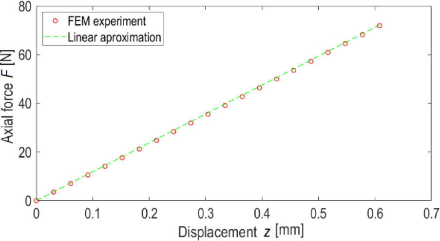
An example plot of the force-displacement curve for a spring with C = 4, na = 1, γ = 10° and s = 0.5, obtained from numerical simulation is shown in Figure 8. It can be noticed that, nonlinearity of force-displacement curve is negligible.
Fig. 8.
Force-displacement curve for a spring with C = 4, na = 1, γ = 10° for coil contact length s = 0.5
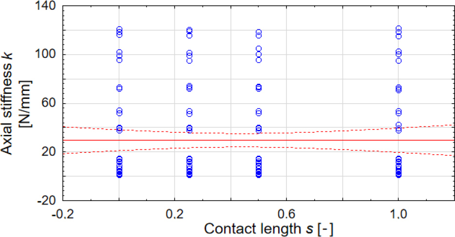
The results of the axial stiffness tests were too extensive to be presented in full in this publication. Therefore, they were aggregated, and the trends in stiffness changes were analyzed. Data analysis began by examining the correlation of the output variable, i.e., numerical axial stiffness k, with the input independent variables C, na, γ, and s, for the primary set of 180 springs. The results of the correlation analyses are presented in Figures 9–12 along with the correlation coefficients.
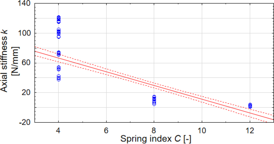
Fig. 10.
Correlation plot of axial stiffness k versus number of active coils na with coefficient r = -0.29
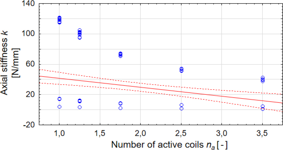
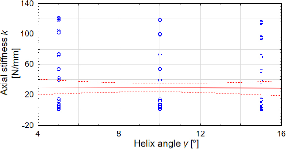
Fig. 12.
Correlation plot of axial stiffness k versus contact length per one ending s with coefficient r = -0.0002
The analysis conducted on the given sample revealed that the axial stiffness is primarily influenced by the input variables used in the classical formula from the standard, namely the spring index C and the number of active coils na. The spring angle γ, included in many more precise formulas, has a significantly smaller effect, while the spring end coil contact length has practically no influence. However, this conclusion needs to be verified for specific spring geometries. To this end, the coefficient of variation was calculated for each of the contact configurations of the coils within the same number of active coils. The coefficient of variation, expressed as a percentage, represents the ratio of the standard deviation to the mean value of the sample. The results are presented in Table 3, with coefficients color-coded for clarity.
Tab. 3.
Coefficient of variation of springs axial stiffness depending on spring angle, number of active coils and spring index
The highest coefficients of variation were obtained for C = 4 and γ = 5°. This aligns with the results from experimental studies for C = 5, where variations in stiffness due to changes in the terminal coil contact length were also evident. For C = 12 the stiffness variability coefficient did not surpass 1%. For C = 8, the coefficient exceeded 0.5% only twice, to values of 0.81% and 0.64%. In general, it is accepted that a feature is statistically significant if the coefficient of variation exceeds 10%. This threshold was not reached. The vast majority of spring sets showed no change in stiffness due to changes in the spring end coil contact length, allowing the conclusion that this factor is insignificant, except for small angles and small spring indices. Therefore, for further calculations, the stiffness value for point contact (s = 0) will be used.
Figure 13 illustrates the change in axial stiffness for springs with point contact and a spring index of C = 8, depending on the number of coils and the spring angle. This confirms the minimal effect of the spring angle on axial stiffness. Additionally, all variability patterns exhibit the same trend: the greater the number of coils, the lower the stiffness. This reflects the fundamental relationship provided in EN 13906-1:2013(E).
Fig. 13.
Axial stiffness for index C = 8, point contact (s = 0) for spring angles of 5, 10 and 15 degrees

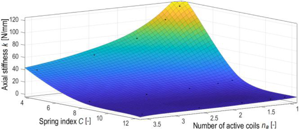
A general overview of the results for point contact of the terminal coils is visualized in Figure 14, created using Matlab. The three axes represent the influence of the spring index C and the number of active coils na on axial stiffness k. The most significant changes in stiffness are observed for low spring indices and small numbers of active coils.
Fig. 14.
Axial stiffness distribution depending on the spring index C and the number of active coils na for the point contact of end coils
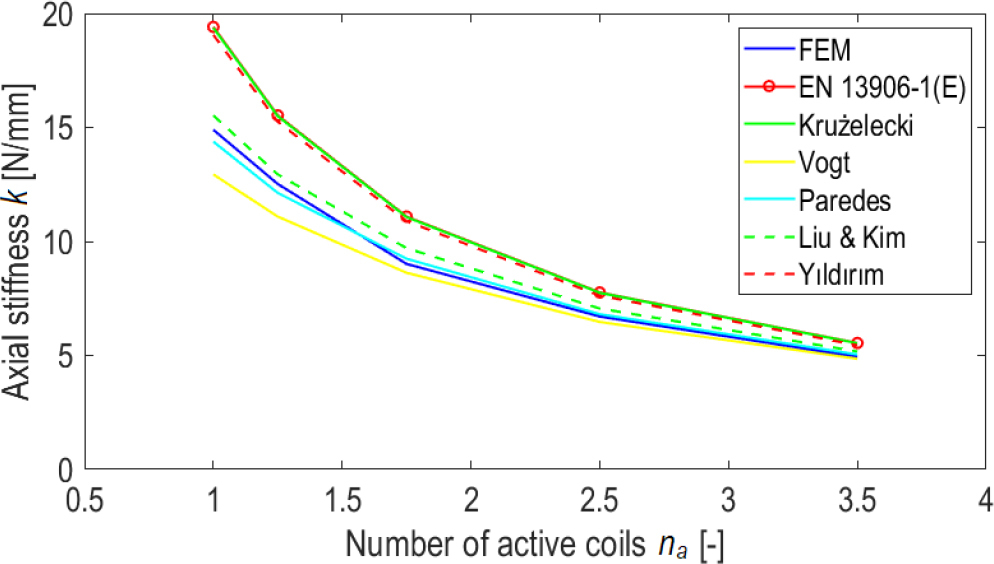
Fitting functions to the data visualized in Figure 14 proved challenging. Consequently, the applicability of formulas described in Section 2 was analyzed, highlighting differences for the batch of springs with C = 8, γ = 5°, and s = 0. The plot given in Fig. 15 indicates that the formulas by Paredes and Liu & Kim, which introduce an equivalent number of active coils, most closely align with the simulation results. Similar results are provided by the formulas from EN 13906-1:2013(E), Yıldırım, and Krużelecki, though they deviate from the FEM results. The Vogt correction produced values close to the simulation outcomes for springs with more than 2.5 active coils. The greater the number of active coils, the more accurate all formulas become.
Fig. 15.
Axial stiffness k for the index C = 8, angle γ = 5°, point contact (s = 0) in comparison with selected analytical methods
A decision was made to derive a new formula based on the most commonly used equation from EN 13906-1:2013(E). To accomplish this, the ratio 𝜒 (Equation 12) between the axial stiffness value obtained using FEM (kFEM) and the value calculated using the standard formula (kN) was computed.
Then, the average value of 𝜒 was calculated for each number of coils, i.e. for 4 measurements of axial stiffness depending on the contact length. Using the Curve Fitting Tool in Matlab, a power function (13) was fitted to the 𝜒 coefficient, which tends to 1. In this way, it was not avoided that the stiffness was significantly higher than the value obtained from the formula in spring norm [25]. This assumption was made because in the vast majority of FEM data, the axial stiffness was lower than the value calculated from the standard formula. The function was made dependent only on the number of active coils. The results of fitting the function (13) to the calculated 𝜒 coefficients are given in Table 4.
Tab. 4.
The values of coefficient a and b of equation (13) depending on the spring index C and helix angle γ together with the given R-square parameter
| C | γ [°] | a | b | R2 |
|---|---|---|---|---|
| 4 | 5 | 4.550 | 0.6462 | 0.8685 |
| 10 | 4.328 | 0.5942 | 0.9889 | |
| 15 | 3.946 | 0.4576 | 0.9917 | |
| 8 | 5 | 4.409 | 0.5350 | 0.9164 |
| 10 | 4.168 | 0.4938 | 0.9726 | |
| 15 | 3.701 | 0.3970 | 0.9961 | |
| 12 | 5 | 4.393 | 0.5183 | 0.9021 |
| 10 | 4.055 | 0.4600 | 0.9751 | |
| 15 | 3.587 | 0.3937 | 0.9910 |
Fitting with the function Eq. (13) appeared to be sufficiently accurate obtaining the lowest R-square of 0.8685, and an average of about 0.956. All data was regular and therefore was used for determining the description of parameters a and b with respect to the spring angle γ. In Matlab, attempts were made to fit various forms of the function, for example, giving high accuracies (of the order of R-square equals 1) Gaussian or Power options, but it was difficult to produce a generalized form describing all the data with high accuracy. The Rational form also gave good results, but contained three parameters. It was decided to use the linear form Eq. (14) and (15) with two parameters to keep the formula as simple as possible.
The values of the parameters k1, k2, m1, m2 are given in Table 5, and the finished formulas are described in equations (16) and (17).
Tab. 5.
The values of coefficient k1 k2, m1, m2 of equations (14) and (15) depending on the spring index with the given R-square parameter
| C | k1 | k2 | R2 | m1 | m2 | R2 |
|---|---|---|---|---|---|---|
| 4 | -0.060 | 4.879 | 0.9771 | -0.019 | 0.755 | 0.9371 |
| 8 | -0.071 | 4.801 | 0.9672 | -0.014 | 0.613 | 0.9487 |
| 12 | -0.081 | 4.818 | 0.9914 | -0.012 | 0.582 | 0.9986 |
| Av. | -0.071 | 4.833 | 0.9786 | -0.015 | 0.650 | 0.9615 |
The average values of a and b were then approximated by equations (16) and (17) which parameters were the average value of k1 k2, m1, m2 in terms of spring index (Tab. 5), determining the R-square of the model. The results of the approximation are recorded in Table 6.
Tab. 6.
Comparison of parameters a and b calculated using equations (16) and (17) with the target values
The calculated R2 values mean that it is possible to approximate these values with the given formula. Other attempts have not yielded a better value in terms of R2. The final form of the formula for the axial stiffness kχ dependent on the kN formula (1) derived from [25] has the form Eq. (18).The developed correction factor reflects the effect of the number of active coils na and the helix angle γ given in degrees.
The formula (18) allows to calculate with high accuracy (above 90%) the axial stiffness of steel springs with an index from 4 to 20, number of active coils from 1 to 5 and helix angle from 5° to 20°. This was checked on a random selection of 6 springs with the mentioned sizes of these parameters obtaining MAPE equal to 2%. Table 7 compares the determined formula (18) with those described in Chapter 2. The mean absolute percentage error (MAPE) was calculated for a sample of 180 springs, which served as a measure for the comparison of results.
Tab. 7.
Comparison of the accuracy of selected methods for calculating the axial stiffness of compression springs
It is showed that the most accurate method is the one with a correction calculated in a power-law manner (18), achieving a MAPE of 1.38%. The least accurate was the formula commonly used described by Eq. (1). Among the known methods, the Paredes method (2) is the most accurate, with a MAPE of 3.62%.
Table 8 shows a comparison of the two most accurate methods and method (1) [25] with the actual axial stiffness values obtained from the experiment performed, described in Chapter 3.
Tab. 8.
Comparison of axial stiffness values calculated using the most accurate methods and the commonly used Eq. (1) with bench test results
Table 8 indicates that the compared formulas are more accurate for larger spring index. Formula (18) achieved a MAPE for C = 5 of 7%, and 2% for C = 7. The smallest mean absolute percentage error (MAPE) was shown by the Paredes formula (2) – 5% and 2%, respectively. For C = 5 and contact s = 0.25, the better accuracy of formula (1) is noted. Due to the fact that the new formulas proposed in the article are subject to numerical simulation error, their accuracy is comparable to commonly used methods. This means that they can be used alternatively. In addition, the real springs were not made with high precision. The methodology used to determine the correction to formula (1) can be successfully applied to determine more accurate formulas on the basis of extensive stand tests. This task is feasible, but the cost of implementation may exceed the expected result. These errors are based on various material and geometric deviations. Therefore, extensive bench testing could only statistically determine an accurate method.
. Transverse reaction value Influence of geometrical parameters on spring response in the transverse direction
The numerical compression simulations conducted on the initial set of 180 spring models allowed conclusions to be drawn regarding the influence of individual geometric parameters on the transverse reaction force exerted by the spring on the support. Based on these analyses, the value of the relative transverse reaction Rrel was determined. This quantity was defined as the ratio of the transverse reaction force of the spring to its axial reaction force during axial compression, under conditions where the displacements of the supports in transverse directions were constrained:
where Rx and Ry are the numerically determined components of the transverse reaction. The angle formed by the resultant vector of the transverse reaction with the X-axis, which marks the start of the spring wire, was also determined. The results of 180 simulations investigating the influence of geometric parameters on the relative transverse reaction value are illustrated by the surface plots shown in Fig. 16.Fig. 16.
Plots of the Rrel dependency on the contact length and the helix pitch angle for springs with a given spring index C and number of active coils na
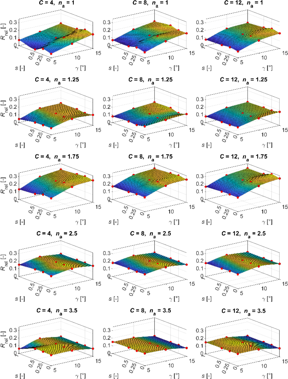
The surface plots shown in Fig. 16 reveal a significant variation in relative transverse reactions Rrel, ranging from values close to zero to those exceeding 0.3. These plots also demonstrate the low degree of correlation between Rrel and the contact length s. This is consistent with the correlation analysis performed earlier, performed analogously to point 4.3.1 for axial stiffness. This analysis showed that: the correlation coefficient r of the transverse reaction value generated during axial compression with the spring index C equals -0.52, with the number of active coils na equals -0.03, with the helix angle γ 0.56 and with the contact length s -0.02. Therefore, the reaction value depends most on the spring index and helix angle. Additionally, the plots indicate that the maximum Rrel values occurred at an active coil count of na = 1.75, regardless of the spring index C. To determine the relationship between Rrel and the number of active coils na, further 45 analyses were conducted by extending the range of active coil counts to: 1, 1.25, 1.5, 1.75, 2, 2.25, 2.5, 2.75, 3, 3.25, 3.5, 3.75, 4, 4.25, 4.5 and 5. Based on observations indicating a minor influence of the contact length s and the spring index C on the variation of Rrel, subsequent analyses were limited to springs with s = 0 and C = 8. The total number of numerical analyses carried out was therefore 225. Fig. 17 presents the results of the relationship between relative transverse reaction Rrel and the number of active coils na for helix angle values γ: 5°, 10° and 15°.
Fig. 17.
Plots of the Rrel dependency on the number of active coils na for helix pitch angles γ: 5°, 10°, 15°, for springs with C = 8 oraz s = 0
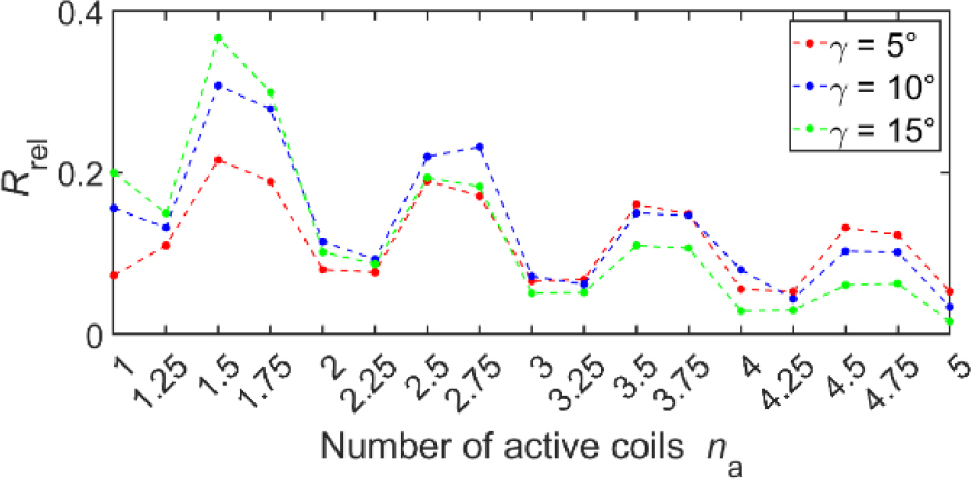
The presented plots clearly show that the highest Rrel values occur for springs with partial coil numbers of 0.5 and 0.75, whereas the lowest relative transverse reaction values are observed for springs with fractional coil numbers of 0 and 0.25. This observation provides an important insight for the spring designers, as it enables the deliberate selection of the active number of coils, which should be chosen not only based on the required axial stiffness but also considering the desired transverse reaction value.
The presented results were utilized to develop a generalized approximation model capable of estimating Rrel values depending on the number of active coils for springs with any spring index C and helix angle γ.
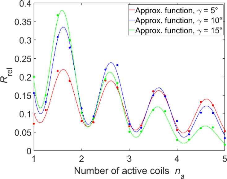
Given the pattern of Rrel variations shown in Fig. 17, resembling a damped sinusoid, functions composed of the product of a decaying nonlinear function representing the mean value trend and combinations of trigonometric functions were tested. Among all the tested functions, the best fit was achieved with the function of the form:
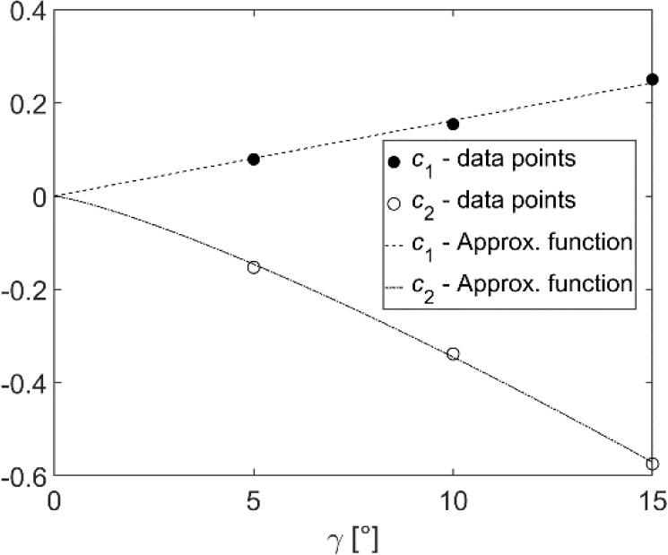
Fig. 18 shows the preliminary approximation functions (continuous lines) along with the input data (dots), while Table 9 provides the values of the obtained coefficients ci and the corresponding coefficients of determination.
Fig. 18.
Preliminary approximation plots of Rrel as a function of the number of active coils na for helix pitch angles of 5° 10° and 15°, for springs with C = s and = 0
Tab. 9.
The values of the function coefficients Eq. (20), along with the coefficients of determination
| γ [°] | c1 | c2 | c3 | c4 | R-square |
|---|---|---|---|---|---|
| 5 | 0.0685 | -0.1508 | 2.7048 | 1.2563 | 0.9862 |
| 10 | 0.1660 | -0.3381 | 2.1928 | 0.8522 | 0.9853 |
| 15 | 0.2731 | -0.5805 | 2.1819 | 0.9409 | 0.9948 |
To achieve a simple and easily applicable relationship, the values of coefficients c3 and c4 have been fixed. Each value was set to the average of all values for the different angles γ: c3 = 2.3598 and c4 = 1.0165. Based on this assumption, another approximation was performed to determine the corresponding values of coefficients c1 and c2. The results are presented in Table 10.
Tab. 10.
The approximation results with fixed values of coefficients
| γ [°] | c1 | c2 | c3 | c4 | R-square |
|---|---|---|---|---|---|
| 5 | 0.0787 | -0.1529 | 2.3598 | 1.0165 | 0.9760 |
| 10 | 0.1541 | -0.3385 | 0.9796 | ||
| 15 | 0.2502 | -0.5745 | 0.9934 |
The final step was to determine the approximation functions for the dependencies c1(γ) and c2(γ) based on the data presented in Table 10. The aim was to find the simplest possible functions that ensure a coefficient of determination not less than 0.99. Ultimately, the approximation of the dependency of coefficient c1 on the helix pitch angle γ was performed using a linear function, while c2 was approximated using a power function:
The coefficients of determination for both approximations were 0.9920 for c1 and 0.9988 for c2, respectively. A graphical representation of the correspondence between input data and approximation functions is shown in Fig.19.
Fig. 19.
Approximation plots of coefficients c1 and c2 along with the data for springs with C = s and = 0
By substituting equations (21a) and (21b) into Eq.(20), we obtain, after transformations, the final relationship which allows to determine the value of Rrel as a function of the number of active coils na and the helix angle γ:
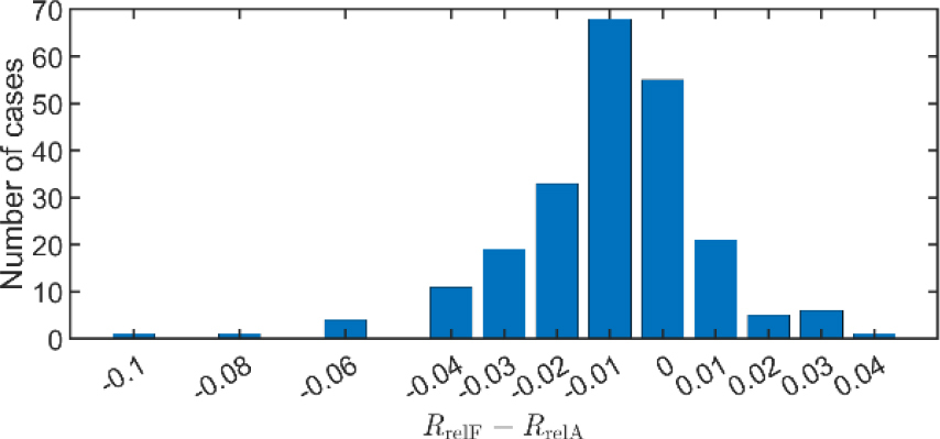
The analysis of the compliance of Eq. (22) with the results of FEM analyses was performed for a full set of 225 geometric spring models. This analysis showed that:
– Only in 6 cases out of 225, the absolute value of the difference between the Rrel determined from the FEM analyses (denoted hereafter as RrelF) and the result of Eq. (22) (denoted hereafter as RrelA) exceeded the value of 0.05;
– In 75 cases out of 225, the absolute value of the difference between RrelF a RrelA was within the range between 0.01 and 0.05;
– In the remaining 144 cases, the value of |RrelF — RrelA| did not exceed 0.01.
A graphical interpretation of the results obtained is shown in Fig.19, where the vertical axis represents the number of cases with a given difference value RrelF — RrelA, while the horizontal axis shows the values of the obtained differences rounded to two decimal places.
It can be seen in Fig. 20 that the absolute value of RrelF — RrelA difference exceeded 0.06, only in 2 cases. All of them refer to springs with index C = 4 and helix angle γ = 5°. It should be noted that the average value of relative transverse reaction Rrel for the set of 225 tested spring models was equal to 0.16, while the average value of RrelF — RrelA difference was only 0.0095, thus it is only about 5.9% of the average Rrel value. The performed analysis indicates the high accuracy of the proposed Eq. (22) over a wide range of variation in the geometric parameters of springs.
. Transverse reaction angle
As shown in section 4.3.2, the value of the transverse reaction generated by the spring during axial compression can reach significant levels. These reactions may be substantial enough that neglecting them during the design of the system in which the spring operates would lead to an oversimplification. One possible solution in such cases is to arrange the springs so that their transverse reactions cancel each other out. For this to be feasible, the designer must have knowledge of the direction of the transverse force to correctly determine the spring assembly. Precise determination of this direction may require simulations or experimental testing. However, the ability to approximate it using a simple relation at an early stage of the design process can be highly beneficial, potentially reducing the number of iterations during the design phase. Based on the analyses conducted, such a relation is presented in this section.
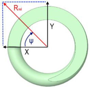
To determine the direction of the transverse reaction, the angle ψ was defined as the angle between the mentioned direction and the X-axis. The reaction angle ψ was calculated relative to the X-axis, as the arcus cosine of the reaction value on the X-axis to the resultant reaction value Rrel. Additionally, the sign of the transverse reaction was included to account for its orientation. For instance, angles of 135° and -45° represent the same direction but opposite orientations. The direction of the resultant reaction was determined based on the plus or minus signs of the reactions on the X and Y-axes. This is illustrated in Fig. 21. The analysis was based on all 225 conducted studies. Similarly to previous analyses, correlations between variables were first examined. The correlation coefficient r of angle with the spring index was -0.005, with the number of active coils -0.179, with the spring angle -0.004, and with end coil contact length -0.063. Thus, it is evident that the direction of the transverse reaction is independent of these parameters.
Fig. 21.
The coordinate system used to determine the transverse reaction angle Rrel. Top view of the spring
The results are presented in Table 11. The values provided in the table are accurate to within +/-3°. For the parameters C = 4 and γ = 5°, which occur simultaneously, deviations from the general trend were observed. These cases were excluded, as previously noted, as challenging spring geometries whose behavior is best evaluated experimentally or numerically.
Tab. 11.
Results of the transverse reaction angle ψ test due to axial compression – basic 225 results
Analyzing Table 11, it was found that the different configurations of the partial number of coils and contact lengths yielded the same values of angle ψ, regardless of the number of coils, helix angle and spring index. In order to describe the course of changes in more detail, 20 additional analyses were carried out for spring models with C = 8, γ = 10°, na = 1, 1.25, 1.5, 1.75 and contact lengths s = 0.125, 0.375, 0.625, 0.75, 0.875. All the values of angle ψ obtained from the FEM analyses are shown in Fig. 22, along with linear approximation functions. Based on these data, equation (23) was derived, describing the course of change of angle ψ as a function of contact length s and the partial number of active coils np.
Fig. 22.
Graph of functions describing the dependence of the transverse reaction angle ψ on the contact length s and the partial number of active coils np
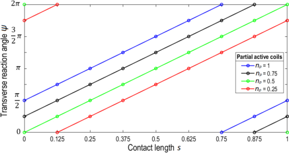
where: np – partial number of active coils. When the number of active coils is an integer, assume that np = 1.
The relationship (23) is valid only for the values of the partial number of active coils listed in Fig. 22, since, as additional tests not included here have shown that in other cases this relationship may not give satisfactory results.
CONCLUSIONS
This article presents an in depth analysis of the changes in axial stiffness, the transverse reaction from axial compression and the angle of this reaction. Also presented is a comprehensive modeling process of spring work in the Static Structural module of Ansys Workbench software, supported by bench tests. The prepared numerical model achieved an accuracy of about 2.7% (MAPE), which allows us to unequivocally confirm the sufficient effectiveness of the use of the finite element method for modeling the basic characteristics of the spring's work.
As a result of numerical experiments of the axial stiffness, it was found that the size of the contact of the end coils does not significantly affect the axial stiffness variance except for the index C = 4 and the spring angle γ = 5° at the same time. A formula (18) was drawn up to calculate the axial stiffness with satisfactory accuracy with a mean absolute percentage error (MAPE) of less than 2% for numerical simulations and from 2 to 7% for real tests. The proposed equation (18) can be used to calculate the axial stiffness of typical coil springs encountered in industry, with an index between 4 and 20 and a helix angle between 5° and 20°, as it gives the most accurate results in this regard among all verified computational models available in the existing literature with respect to the numerical analyses performed. This is especially true for short springs with a small number of active coils. The consistency of formula (18) with the results of numerical analyses was verified only for springs with the number of active coils from 1 to 5. However, as the number of active coils increases, the value of the correction factor in parentheses in Eq. (18) approaches unity. It follows that relation (18) can be used for springs with any number of active coils, not less than 1. It was also pointed out that the Paredes method proposed in 2016 achieves very good agreement at a similar MAPE level of 2 to 5%. The construction of an accurate formula can only be based on bench tests on a large sample of springs.
Numerical studies have made it possible to address an issue not addressed in the previous literature, which is the occurrence of transverse reaction, generated during axial compression of the spring. The numerical studies carried out in this paper allowed to formulate new relations in this regard. The relation (22) proposed in Section 4.3.2 is easy to apply and allows to estimate the value of the transverse reaction force arising in axial compression of the spring. Numerical studies have shown that this force can exceed up to 30% of the value of the axial force. In engineering practice, it is important to know not only the values of transverse reaction forces when springs are axially loaded, but also the directions of their action. This allows for an informed selection of the orientation of springs in machine support systems, in order to achieve adequate stability of a given system. In this paper, an analysis of the dependence of the direction of the transverse reaction on the shape of the end coils and on the number of active coils was carried out. This analysis made it possible to propose a new relation (23) to determine this angle. The values of the angle turned out to be reproducible for all springs depending on the partial number of active coils and the number of contacting coils with an accuracy of +/-3°. This rule was not observed for small spring index C < 5 and simultaneously occurring spring angle γ < 10°, which is due to the large curvatures and the close position of the coils relative to each other. The map produced and the formula describing it are simple enough to give results with the same accuracy as the input data (+/-3°). These results are an important input for simplifying the design of compression springs and their installation, since they cover the most commonly used geometries, i.e. with faces ground to ¾ of the circumference, commonly occurring spring angles and spring indexes.