
INTRODUCTION
Steel-concrete composite beams are widely used structural elements in mechanical and structural systems, where time‑varying loads often induce vibrations [1] that affect performance [2] or safety [3]. Accurate prediction of their dynamic behavior has driven the development of various analytical and numerical modeling technique which offers complementary approaches for dynamic analysis of steel-concrete composite beams [4].
Analytical beam models remain popular due to their simplicity and the availability of closed-form or simplified numerical solutions. The classical formulation introduced by Euler and Bernoulli [5] assumes perfect bonding and neglects shear deformation and rotary inertia, leading to overestimated stiffness and natural frequencies, especially in short-span or thick composite beams. Timoshenko’s refinement [6] addresses these limitations by incorporating shear flexibility and rotary inertia, providing more accurate frequency predictions for stocky members while maintaining a relatively simple mathematical form. More advanced approaches, such as Reddy’s higher-order theory [7], relax the rigid cross‑section assumption by introducing a cubic in‑thickness displacement field, allowing cross‑sectional warping and a more realistic shear stress distribution. This increased fidelity, however, comes at the cost of more complex governing equations that often lack closed‑form solutions and require numerical techniques for implementation [8].
One example of steel-concrete composite beams analyzed using analytical models are beams consisting of a steel section with a reinforced concrete slab resting on it, as presented in the work of Berczyński and Wróblewski [9]. Authors investigated the free vibrations of steel-concrete composite beams consisting of a rolled IPE 140 steel beam connected to a reinforced concrete slab via steel stud connectors. Three analytical models were developed: two based on Euler beam theory, which included partial shear connection effects but assumed rigid cross-sections and neglected shear deformation and rotary inertia, and one based on Timoshenko beam theory. The latter accounted for shear flexibility and rotary inertia of the composite cross-section, leading to much closer agreement with experimental natural frequencies, particularly for higher vibration modes. The study demonstrated that including shear and rotational effects significantly improves dynamic modeling accuracy. These studies were later continued [10], where three composite beams with different connection stiffness were tested experimentally, and the Timoshenko model was complemented by a discrete rigid finite element model, both of which were successfully validated against modal test data and used to identify connection stiffness parameters.
Other researchers have extended analytical modeling to damage detection. Dilena and Morassi [11] proposed an analytical method for damage detection in steel-concrete composite beams based on vibration measurements. The authors developed an Euler-Bernoulli beam model incorporating a shear-type connection to represent partial interaction between steel and concrete, enabling the prediction of natural frequencies and mode shapes for both undamaged beams and those with partially degraded shear connectors. The model was experimentally validated through dynamic tests on specimens in both undamaged condition and with varying levels of connector damage, showing good agreement with the measured natural frequencies and mode shapes, including for intermediate damage states. To enhance modeling accuracy, the authors also derived a refined version of the model based on Timoshenko beam theory. The method successfully identified the location and severity of damage through frequency shifts, although its sensitivity decreased for low damage levels.
Continuous analytical models provide an efficient means for predicting the global dynamic behavior of steel–concrete composite beams, offering fast evaluation of natural frequencies and mode shapes. Although well-suited for simplified geometries and boundary conditions, these models rely on idealized assumptions that limit their ability to accurately capture local phenomena such as interface slip, material discontinuities, and cross-sectional warping.
In parallel with analytical beam theories, numerical modeling techniques based on the finite element method [12] and its derivatives, including reduced‑order models [13] and rigid finite element formulations [14], have become standard tools for analyzing steel-concrete composite beams. These methods, particularly the finite element method, enable detailed representation of complex geometries, material interfaces, and connection conditions, making them particularly suitable for layered or infilled structures.
Shen et al. [15] proposed a component‑wise analytical approach based on the Carrera unified formulation [16] to study free vibration and stress analysis of steel–concrete composite beams. The method discretized the beam cross‑section using Lagrange polynomials of different orders and allowed each material component to be modeled separately while automatically enforcing interfacial continuity. Closed‑form Navier‑type solutions were derived for simply supported beams and validated on I‑ and box‑section steel-concrete composite beams. The results showed that the Carrera unified formulation component‑wise approach can achieve three‑dimensional accuracy in natural frequencies, mode shapes, and stress fields with significantly fewer degrees of freedom compared with full 3D finite element models. The main limitations include the assumption of perfect bonding between steel and concrete, linear elastic material behavior, and the focus on simple boundary conditions.
Henriques et al. [17] proposed a Generalized Beam Theory (GBT)-based finite element model for the dynamic analysis of steel-concrete composite beams [18], incorporating concrete cracking and cross-section deformation effects, including shear lag. The approach involves a two-step procedure: an incremental static analysis to account for non-linear behavior and to obtain the tangent stiffness matrix, followed by an eigenvalue analysis to compute natural frequencies and vibration mode shapes. The method makes use of GBT modal decomposition to represent structural deformation through a set of predefined cross-section modes, enabling reduced-order modeling with lower computational cost. The model was applied to simply supported beams subjected to uniform and eccentric loading, and the results were compared with those obtained from shell finite element models. Good agreement was observed in terms of natural frequencies and mode shapes, with significant reduction in the number of degrees of freedom. The method was also able to capture the influence of cracking on modal behavior. Limitations include simplified assumptions regarding concrete material behavior and the treatment of shear connection.
Assem et al. [19] proposed a refined quasi‑3D beam theory combined with the differential quadrature finite element method to analyze free vibration of steel box‑section beams infilled with porous polymer concrete cores. The study introduced different porosity distributions (uniform and two non‑uniform patterns) and investigated their effects on natural frequencies under various boundary conditions and slenderness ratios. The model demonstrated high accuracy compared with experimental data and highlighted that strategically non‑uniform porosity can maintain stiffness while reducing mass. However, the analysis assumed ideal material behavior and lacked experimental validation of porosity‑specific configurations. In a subsequent study, the authors extended the proposed quasi-3D DQFEM framework to investigate the influence of crack presence and location on the dynamic behavior of composite steel–polymer concrete box-section beams [20].
The rigid finite element method [21] provides a reduced-order modeling approach for the dynamic analysis of steel-concrete composite beams. In this formulation, the structure is discretized into rigid segments interconnected by translational and rotational springs, efficiently capturing deformability while significantly reducing the number of degrees of freedom compared to conventional finite element models.
Abramowicz et al. [22] developed a three-dimensional rigid finite element model for steel-concrete composite beams, enabling analysis of flexural, torsional and distortional vibration modes that cannot be captured by conventional two-dimensional approaches. The model separately represents the concrete slab and steel I-section, linked by spring-damping elements to realistically reproduce connector dynamic properties. Dynamic tests were performed on two beams with different connector spacings, and model parameters (e.g., connector stiffness and equivalent longitudinal modulus of the concrete slab) were identified using natural frequencies and mode shapes from impulse response experiments. The validated model showed good agreement with experimental results and was applied to simulate connector damage, demonstrating the feasibility of vibration-based damage detection for composite structures
Dunaj et al. [23] applied the rigid finite element method to model the dynamic behavior of a steel beam filled with polymer concrete, aiming to provide a low‑dimensional yet accurate alternative to conventional finite element models. The proposed approach aggregated the mass and stiffness of steel and polymer concrete into discrete rigid elements connected by spring‑damping elements, enabling efficient calculation of natural frequencies, mode shapes, and frequency response functions. Modal testing confirmed good agreement in terms of mode shapes and natural frequencies, while the model significantly reduced computational complexity compared to full 3D FEM simulations. Reported limitations include reduced accuracy in predicting non-resonant frequency response.
The reviewed literature indicates that continuous analytical models and finite element models offer complementary strengths and limitations in the dynamic analysis of steel-concrete composite beams. Continuous models provide closed-form expressions for natural frequencies and mode shapes with minimal computational effort. They are well suited for parametric studies, damage detection, and theoretical investigations but rely on simplifying assumptions such as perfect bonding, uniform cross-sections, and linear material behavior, which may limit their applicability to complex or layered structures. Conventional finite element models, in contrast, offer high accuracy and flexibility, allowing detailed representation of material interfaces, geometry, and boundary conditions. However, this comes with increased computational cost and greater modeling complexity. The rigid finite element method provides a reduced-order alternative by discretizing the structure into rigid segments connected by translational and rotational springs [24]. This approach enables an efficient representation of deformability, particularly useful for capturing partial shear interaction and interface slip, while significantly reducing the number of degrees of freedom. Its limitations include reduced accuracy in modeling non-resonant dynamic behavior and the use of simplified, often isotropic, material properties.
Although considerable progress has been made in modeling the dynamic behavior of steel-concrete composite beams, certain aspects remain the subject of ongoing development. In particular, comprehensive continuous analytical models that account for all fundamental vibration modes – transverse, longitudinal, and torsional – and enable the evaluation of amplitude-frequency response characteristics are still limited. To contribute to this area, the present study proposes a continuous analytical model for thin-walled box-section beams filled with polymer concrete, which captures transverse, longitudinal, and torsional vibrations. The equations of motion are derived using Hamilton’s principle, ensuring a consistent formulation grounded in energy methods. By incorporating damping, the model enables direct evaluation of frequency response functions, providing a more complete dynamic characterization. The homogenized formulation adopted in this study enables efficient evaluation of global dynamic characteristics while maintaining sufficient accuracy, which makes it particularly suitable for parametric analyses and iterative computational procedures, where component-wise models would lead to significantly higher computational cost. The proposed model has been experimentally verified and validated using reference data from the literature, confirming its suitability for analyzing the vibration performance of steel-polymer concrete composite beams.
The paper is organized as follows: Section 2 introduces the research object, a steel-polymer concrete beam, and its static and dynamic experimental testing. Section 3 presents the modeling methodology, including key assumptions and formulations. Section 4 reports the results, verifying the proposed modeling approach and comparing its accuracy with alternative methods from the literature. Section 5 discusses the findings, and Section 6 concludes with key insights, limitations, and directions for future work.
MATERIALS AND METHODS
Research object
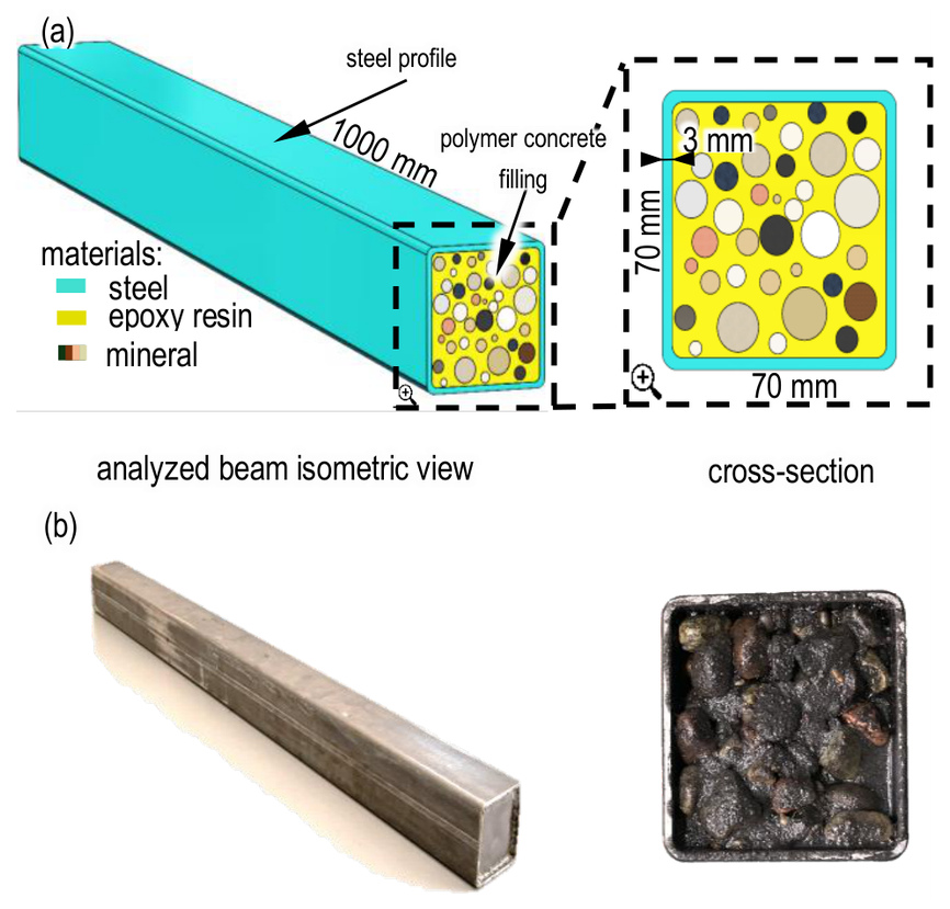
The research object is a steel-polymer concrete beam designed to combine the stiffness of steel with the vibration-damping capability of polymer concrete. The analyzed beam used a square steel profile with a cross-section of 70 × 70 mm, a wall thickness of 3 mm and a length of 1000 mm. The profile was filled with polymer concrete and compacted to ensure complete filling. The polymer concrete composition, based on previous studies [25,26], consisted of epoxy resin and mineral aggregates of various grain sizes. The aggregates were divided into fractions according to grain size: ash, a fine fraction (mainly sand, 0.25-2 mm), a medium fraction (2-10 mm), and a coarse fraction (8-16 mm, primarily irregularly shaped gravel). The mass percentages of individual fractions are presented in Tab. 1. The structure of a steel-polymer concrete beam is shown in Fig. 1.
Static tests
Static compression tests were performed to determine the material constants required for modelling. Cuboidal samples of steel (50 × 50 × 110 mm) and polymer concrete (45 × 45 × 110 mm) were tested on an Instron 8850 machine (Instron, Norwood, MA, USA) under controlled laboratory conditions (23 °C, 50 % relative humidity). The setup included a class 0.5 load cell (250 kN capacity) and a class 0.2 Instron 2620‑603 tactile extensometer with measuring ranges of 25 mm and 12.5 mm (±1 mm). Samples were conditioned for 72 h prior to testing. Material properties with associated standard uncertainties and the loss factor, determined from dynamic tests using the half‑power method, are presented in Tab. 2.
Dynamic tests
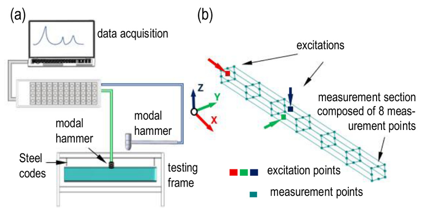
Experimental modal analysis was performed to determine the modal parameters of the manufactured beams, both empty and filled with polymer concrete. Free boundary conditions were approximated by suspending the beams on steel cables, with suspension points (100 mm from each end) and cable stiffness chosen to reproduce natural vibration modes within the target frequency range.
The measurement setup was designed to capture at least the first five deformable vibration modes (20-2600 Hz). Impulse excitation was applied using a PCB 086C01 (PCB Piezotronics, Depew, NY, USA) modal hammer with a polymer tip, providing sufficient bandwidth. To capture transverse, torsional, and longitudinal responses, excitation was applied in three perpendicular directions (+X, −Z, −Y); torsional modes were additionally identified by off‑axis excitation in the −Z direction. Excitation points were selected to avoid nodal regions, located approximately 420 mm from the beam end for Z and Y excitations, and at the closed end for X‑direction excitation.
Responses were measured using eight ICP PCB 356A01 (PCB Piezotronics, Depew, NY, USA) piezoelectric accelerometers mounted simultaneously sing wax as the adhesive. Three‑axis measurements were taken at eight points in each of seven successive sections, resulting in 56 measurement locations. The sensors were repositioned sequentially to ensure complete spatial coverage. The parameters of the impact testing measurement system components are presented in Tab. 3.
Tab. 3
Experimental equipment parameters
Measurement signals were processed using a Scadas Mobile Vibco system with Simcenter LMS Testlab software (Siemens AG, Munich, Germany). Sampling was performed at 8,192 Hz with a frequency resolution of 0.25 Hz. Each transfer function was estimated from 7 repeated excitations using the H1 estimator, and signals were recorded for 4 s, allowing the response to decay without windowing.
CONTINUOUS MODEL OF BEAM VIBRATIONS
Model assumptions
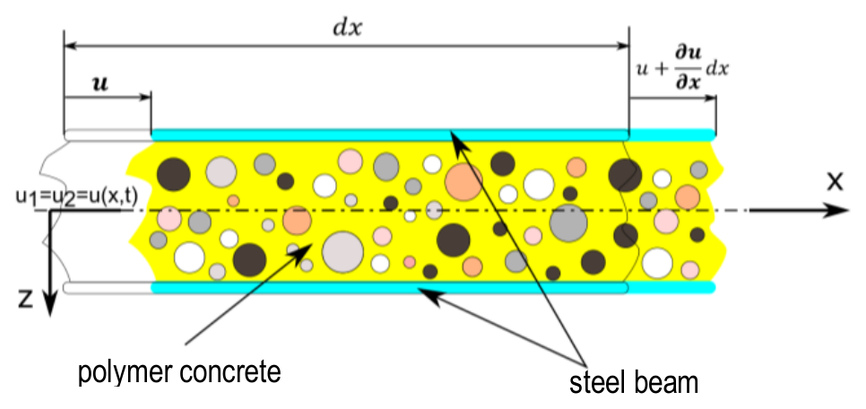
Based on experimental observations, several simplifications were adopted to develop the mathematical model of the beam. Despite the heterogeneous structure of polymer concrete, its dynamic behavior was represented by a linear elastic material model. This assumption was supported by experimental results demonstrating compliance with Maxwell’s reciprocity principle, linear stiffness characteristics and symmetric mode shapes obtained from impulse testing, as detailed in [27,28]. Perfect contact between the steel profile and the polymer concrete filling was assumed along the entire internal surface, with adhesion preventing tangential slip at the interface.
Longitudinal vibrations
The longitudinal vibration model was derived using Hamilton’s
principle, assuming that the deformation of the cross-section in the
transverse directions (

Using the total equivalent coefficients, the potential
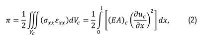

From equations (2) and (3), the equivalent coefficients for a
composite beam can be determined as the sum of the stiffness and mass
coefficients of its individual components sharing a common neutral
axis. The longitudinal stiffness


Applying Hamilton’s principle, the equation of motion of the beam
along the

Assuming a separable solution, the equation can be written as:

where

where:

The function

where the integration constants

Substituting the boundary conditions into equation (10) yields the frequency equation, whose solution gives the natural frequencies:

for which the solutions take the form

where
Assuming the orthonormality condition:

The normalized rigid and flexible longitudinal mode shapes were obtained as:


Torsional vibrations
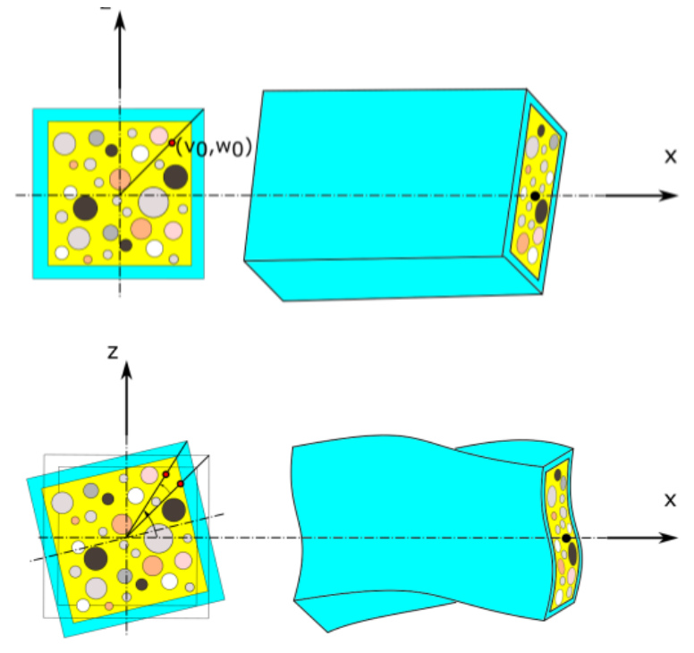
Because the analyzed beam has a cross-section symmetric about both
principal axes, torsion can be treated as independent of other
vibration modes. However, due to the square cross-section, distortion
occurs during twisting. To account for this effect when determining
torsional natural frequencies, the de Saint Venant model was applied,
including a correction for displacement caused by cross‑section
warping. Introducing the warpage function

where
The potential and kinetic energies of the composite beam are given by:
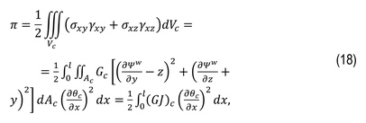
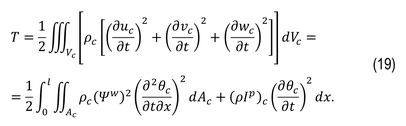
where


where

Assuming a separable solution, the equation can be written as:

where

where:

The function

where the integration constants

Substituting the boundary conditions into equation (26) yields the frequency equation, whose solution gives the natural frequencies:

for which the solutions take the form

Assuming the orthonormality condition:

The normalized rigid and flexible torsional mode shapes were obtained as:


Transverse vibrations
To derive the equations of motion using Timoshenko’s theory, the displacement variables were defined as:

where
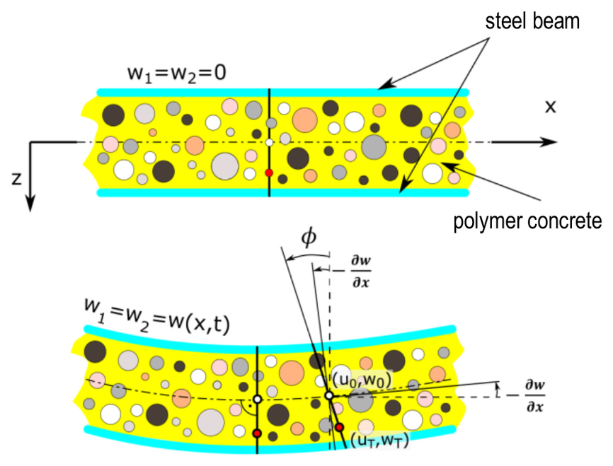
Fig. 5. Longitudinal cross-section of a polymer-concrete beam under bending, showing undeformed and deformed shapes according to Timoshenko’s theory
The shear coefficient
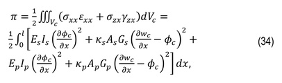
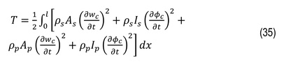
For free vibrations, external forces are absent; hence, the work of external forces is zero.
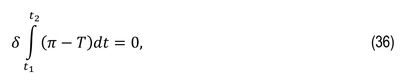
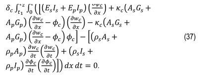
From equations (36) and (37), the equivalent coefficients for
composite beams can be determined from the flexural stiffness



Using integration by parts and grouping terms, the equation for a
uniform beam can be expressed as a system of two differential
equations in terms of the displacement

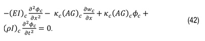
The general solution of these equations for natural vibrations can be written as:

where


where:



After variable separation, the transverse vibration mode functions
for

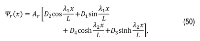
where
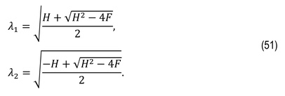
The four integration constants
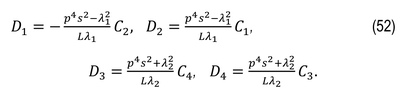
The constant

where the natural vibration mode vector and mass matrix are given by:


The integration coefficients


Using all four boundary conditions and the relationship between the

To solve the system of equations (58), the determinant of matrix


Damping
To determine the system response to excitation, damping was
included in the model. A constant damping coefficient was assumed for
the entire frequency range using a hysteretic model. Starting from the
distributed internal viscous damping relationship [32] in Hamilton’s
principle and considering the Rayleigh dissipation function


To account for internal damping in the continuous model, the composite longitudinal and transverse stiffnesses were assumed as:


The general equation of motion for forced vibrations of a uniform cross‑section beam with damping is written as:

Forced vibration problems can be solved using the eigenfunction superposition method or a closed‑form solution.
RESULTS
Steel-polymer concrete beam parameters
The analyzed beam features a square hollow steel section with an external cross-section of 70 × 70 mm, wall thickness of 3 mm, and total length of 1000 mm. The internal volume is completely filled with polymer concrete. The effective material and geometric parameters of the composite section were determined using classical homogenization rules and are listed in Tab. 4.
Tab. 4
Material and cross-sectional parameters used in the model
The shear coefficient
Experimental verification of mode shapes and natural frequencies
To verify the predictive capability of the developed continuous
model, a comparison was carried out between the calculated and
experimentally measured natural frequencies. The analysis included
transverse, torsional, and longitudinal modes to evaluate the model’s
ability to capture diverse types of vibrational behavior. The accuracy
of the predictions is presented in Tab. 4, which summarizes the
results for the test specimen described in Subsection 2.1 – a square
steel beam with a 70 × 70 mm cross-section, 3 mm wall thickness, and a
total length of 1000 mm. Tab. 5 includes relative error values
Tab. 5
Comparison of experimental and predicted natural frequencies for the 70 × 70 mm, 3 mm wall, 1000 mm long beam
The comparison presented in Tab. 5 confirms full agreement of mode shapes, indicating that the developed model accurately captured the first eleven modes of the composite beam. The predicted natural frequencies match the experimental results with a mean relative error of 0.7 % and a maximum deviation of 2.2 %, observed for the first longitudinal mode (mode 8). Transverse modes, which dominate the dynamic response, were reproduced with high precision, with several modes (modes 4 and 7) showing zero error and others deviating by less than 0.6 %. Torsional modes were slightly underestimated, with relative errors below 1.5 %, while longitudinal behavior was less accurately captured. Overall, the results confirm the suitability of the continuous model for predicting global dynamic characteristics across multiple mode types.
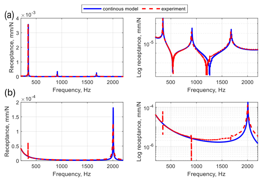
Frequency response functions for both the experimental setup and the model were plotted. Excitation was applied at 7/12 of the beam length from one end, and responses were measured at 2/12 of the length. Fig. 6 presents the linear and logarithmic receptance functions of the analytical model compared with those of the tested beam.
As shown in Fig. 5, the measured and predicted receptance functions display very similar resonance peaks and frequency locations. The agreement in amplitude and curve shape indicates that the developed continuous model provides a reliable approximation of the dynamic response of the tested beam in both transverse directions.
Comparison with Other Modeling Approaches
To further evaluate the applicability of the proposed continuous
model, its results were compared with those obtained using alternative
modeling approaches and with data reported for beams of different
dimensions. This comparison serves as an additional form of
validation, assessing the model’s ability to predict dynamic
properties beyond the specific geometry tested experimentally. It also
highlights the model’s performance relative to other commonly used
analytical and numerical methods. Tab. 6 presents a comparison between
the developed continuous model and two finite element-based
approaches: (i) a one-dimensional beam element model (based on a
classical beam theory) and (ii) a full three-dimensional finite
element model, both reported in [23]. Tab. 6 has been supplemented
with relative error values referenced to the experimental results. The
notation is as follows: δ denotes the relative error for the proposed
continuous model,
The results in Tab. 6 highlight the differences in predictive accuracy between the continuous model and the two finite element approaches. The continuous model achieved a mean relative error of 2.4 %, closely matching the experimental frequencies and demonstrating consistent performance across both transverse and torsional modes. The full three-dimensional finite element model showed slightly better accuracy, with an average error of 1.9 %, reflecting its capacity to capture detailed geometric and material characteristics. In contrast, the one-dimensional beam element model exhibited the largest deviations, with an average error of 4.2 %, particularly underestimating torsional and higher-order transverse modes – a characteristic limitation due to its foundation in Euler–Bernoulli beam theory. These findings suggest that while 3D finite element models offer the highest fidelity, the continuous model provides a favorable balance between accuracy and computational efficiency, outperforming the conventional one-dimensional approach. However, to fully substantiate this observation, a direct comparison with a one-dimensional model based on Timoshenko beam theory would be necessary.
Tab. 6
Comparison of experimental and finite element models-predicted natural frequencies for the 50 × 50 mm, 2 mm wall, 1000 mm long beam
An additional comparison was conducted using data from the
previously referenced study [23], involving a steel-polymer concrete
beam modeled with the rigid finite element method. The results are
presented in Tab. 7, where
Tab. 7
Comparison of experimental and rigid finite element models-predicted natural frequencies for the 50 × 50 mm, 2 mm wall, 1000 mm long beam
The results indicate that both the developed continuous model and the rigid finite element method provide good agreement with the experimental natural frequencies for the steel-polymer concrete beam. The rigid finite element model demonstrated slightly better overall accuracy, with an average relative error of 1.8 %, compared to 2.4 % for the continuous model. This difference is particularly evident in the higher-order transverse modes (modes 6 and 7), where the rigid model achieved errors as low as 0.5 %, while the continuous model showed consistent deviations of 2.6 %.
For the lower-order transverse modes (modes 1 to 4), both modeling approaches performed similarly, although the rigid finite element model produced slightly smaller errors in most cases. In contrast, the continuous model was more accurate in predicting the first torsional mode (mode 5), with a relative error of 2.4 %, compared to 4.1 % for the rigid model. This suggests that while the rigid finite element formulation is well suited for capturing bending-dominated behavior, it may be less effective in describing torsional dynamics.
In summary, the rigid finite element model showed marginally higher accuracy in predicting transverse vibration modes, particularly at higher frequencies, while the continuous model provided more consistent results across both bending and torsional modes.
Based on another study [27], a comparison of natural frequencies
for a 140 mm × 140 mm beam with a 6 mm wall thickness and 1000 mm
length was also conducted. The results, including relative errors
Tab. 8
Comparison of experimental and rigid finite element models-predicted natural frequencies for the 140 × 140 mm, 6 mm wall, 1000 mm long beam
The results presented in Tab. 8 show that the developed continuous model predicted natural frequencies with relative errors ranging from 0.5 % to 2.5 %, with an average of 2.0 %. The three-dimensional finite element model showed slightly higher deviations from 1.0 % to 3.2 %, averaging 2.5 %. For the first and second transverse modes (modes 1, 2, 4, and 5), the continuous model exhibited relative errors of approximately 2.2-2.5 %, while the three-dimensional model showed slightly higher discrepancies. The torsional mode (mode 3) was predicted with the highest accuracy by both models, showing the lowest error levels. This suggests that both modeling approaches capture torsional stiffness reliably.
Discussion
The presented results collectively demonstrate that the developed continuous analytical model offers reliable predictive capability for the dynamic behavior of steel-polymer concrete composite beams across a range of cross-section dimensions and mode types. In all analyzed cases, the model consistently reproduced the experimentally measured natural frequencies with relative errors typically below 3 %, and with a mean error ranging from 0.7 % to 2.4 %, depending on the specific geometry.
The agreement between experimental and predicted receptance functions (Fig. 6) further supports the capability of the continuous model to reproduce not only natural frequencies but also the overall dynamic response of the composite beam. A slight discrepancy in the anti-resonance depth can be observed, which may be attributed to the simplified damping representation adopted in the analytical model.
When compared to high-fidelity three-dimensional finite element models, the continuous model achieved similar or slightly better accuracy in some configurations, particularly for torsional modes and beams with thinner walls. This highlights its ability to efficiently capture global vibrational characteristics without the need for large-scale numerical discretization. While three-dimensional models offer detailed representation of geometry and material interfaces, they do so at significantly higher computational cost. The continuous model, by contrast, provides a valuable trade-off between accuracy and simplicity, particularly in early-stage design, sensitivity studies, or parameter optimization.
Additionally, comparisons with reduced-order modeling approaches such as the rigid finite element method confirmed the robustness of the continuous model. Although the rigid finite element model demonstrated slightly better accuracy in higher-order transverse modes, it also exhibited larger errors in torsional modes. These findings reinforce the observation that the continuous formulation delivers a more balanced representation of bending and torsional behavior – an important feature when dealing with composite beams where both stiffness contributions play a significant role.
The comparative analysis against one-dimensional finite element beam element models based on classical beam theories further underscores the limitations of simplified formulations. The classical approach systematically underestimated torsional and higher-order transverse modes, confirming that such models may not be adequate for vibration analysis of filled sections, particularly when shear deformation and warping effects appear to be significant.
Finally, results obtained for a beam with decreased and increased cross-sectional dimensions (50 × 50 mm, 2 mm wall thickness and 140 × 140 mm, 6 mm wall thickness) confirmed the scalability of the continuous model. Despite substantial differences in cross-section-to-length ratio, the model retained high predictive accuracy.
In summary, the continuous model demonstrated broad applicability, high accuracy, and robustness across different cross-section dimensions. Its performance compared favorably with established finite element methods and reduced-order techniques, supporting its use as an efficient and reliable tool for predicting the dynamic behavior of steel-polymer concrete beams.
CONCLUSIONS
This study presented a continuous analytical model for predicting the dynamic behavior of thin-walled steel box beams filled with polymer concrete. The formulation incorporates transverse, torsional, and longitudinal vibrations, enabling the calculation of natural frequencies and mode shapes. Experimental validation demonstrated that the model accurately predicted the first eleven modes, achieving an average relative error below 1.0 % and full agreement in mode shapes.
Comparative analyses with full three-dimensional finite element models, one-dimensional finite element beam models, and rigid finite element formulations confirm the model’s competitive accuracy. In particular, the proposed approach matched the fidelity of high-resolution numerical models in bending and torsional modes, while offering reduced computational complexity.
The main limitations of the model stem from the assumption of perfect bonding between the steel shell and polymer concrete core, as well as the reliance on homogenized material properties. These simplifications may affect predictions in cases where interfacial slip, local stress concentrations, or heterogeneous infill properties play a significant role.
Future research will focus on extending the model to account for variable cross-sections, non-uniform, or graded infill materials, and damping characterization to enable complete frequency response prediction. Integration into optimization frameworks (benefiting from the significantly lower computational cost compared to detailed 3D FEM models) is also planned to support efficient design of steel-polymer composite structures.