INTRODUCTION

Modern technologies have made it possible to create a variety of coatings that protect the surface of the substrate from harmful damage caused by wear, temperature, or corrosion [1,2]. Applying a uniform coating to the substrate leads to a sharp mismatch in thermophysical properties at the phase boundary, which often makes the coating-substrate interface susceptible to damage, mainly due to high stress concentrations, weak bond strength, and brittleness of the coating materials. An innovative way to eliminate this defect is to use functionally graded materials (FGM), which are characterized by smooth changes in properties across the thickness of the coating [3,4]. FGM coating is used as a inhomogeneous layer between the main homogeneous coating and the substrate, or as a inhomogeneous coating applied directly to the substrate.

Unlike homogeneous coatings, analytical and numerical methods for solving problems of mathematical physics (in particular, thermal conductivity, elasticity, and thermoelasticity) for FGM coatings are complicated by the fact that the differential equations describing such problems contain variable coefficients. The use of classical solution methods is only possible when the change in material properties along the thickness is described by specially selected functions (most often power or exponential) [5 - 7]. However, FGM coatings are a class of composite materials with a representative cell in which two or more phase materials with contrasting properties are combined. The volume fraction of the phase components varies from one coating surface to another. This leads to a inhomogeneous microstructure described by functions that arise as a result of the homogenization procedure. This fact minimizes the applicability of classical methods, and a number of approximate approaches have been developed to overcome the difficulties that have arisen.

Well-known analytical-numerical methods are based on the use of integral transformations Fourier (two-dimensional and three-dimensional problems) or Hankel (axisymmetric problems). The boundary value problems for ordinary differential equations arising in the space of transform is solved using approximate approaches. The most common algorithm for constructing an approximate solution in the literature is to replace FGM coating with continuously changing properties with a package of homogeneous or inhomogeneous layers. An analytical solution of differential equations is constructed in each layer. This approach was first implemented, apparently, in [8]. A two-dimensional frictionless contact problem of elasticity theory for a functionally graded coated half-space was considered. The coating shear modulus was described by an arbitrary continuous function. The Poisson's ratio was considered constant. In each layer of the package, the shear modulus was approximated by a linear function. Similarly, a two-dimensional contact problem with friction [9 - 12], an axisymmetric contact problem [13 - 16], and Reissner–Sagoci problem [17] were solved.

The proposed approach can be used to solve only those problems in which it is possible to construct analytical solutions for the layers that replace the inhomogeneous coating. Therefore, when solving two-dimensional problems, the Poisson's ratio in each layer took a constant value, and in axisymmetric problems, this value was equal to 1/3 [13 - 16]. A more universal approach is one in which all layers in the package are homogeneous. Based on this assumption, a two-dimensional quasi-stationary problem of thermal conductivity [18] and thermoelasticity [19, 20], a three-dimensional elastic problem [21, 22], and an axisymmetric thermoelastic problem [23] were solved.

An alternative to replacing the FGM coating with the package of layers is the numerical solution of the boundary value problem arising in the space of transform. Two algorithms for constructing an approximate solution are known. The first consists in replacing the derivatives in the differential equations and boundary conditions with known difference formulas [24]. The problem is reduced to a system of linear algebraic equations, the solution of which is the value of the transforms of the desired functions at selected nodes. The starting point of the second approach is the approximation of the unknown state functions and their derivatives in the direction perpendicular to the coating surface by certain modeling functions. The structure of these functions is similar to the structure of the analytical solution in the homogeneous substrate. The approach is demonstrated on the example of the axisymmetric heat conduction problem [25]. The boundary value problem is reduced to the initial problem for a system of two ordinary differential equations, which is solved by the Runge-Kutta method.

The intention of this work is to compare the approaches described in the literature. The analysis is carried out on the example of an axisymmetric heat conduction problem, which describes local heating of the body surface with the FGM coating. 5 algorithms are considered. The first three consist in replacing the coating with the continuously changing properties by the package of homogeneous (algorithm A1) or inhomogeneous layers, the thermal conductivity coefficients of which are described by linear (algorithm A2) or exponential functions (algorithm A3). In the algorithm B1, derivatives are replaced by difference formulas [24]. The algorithm B2 uses the approach [25]. The strengths and weaknesses of each of the algorithms are indicated.

FORMULATION OF THE PROBLEM

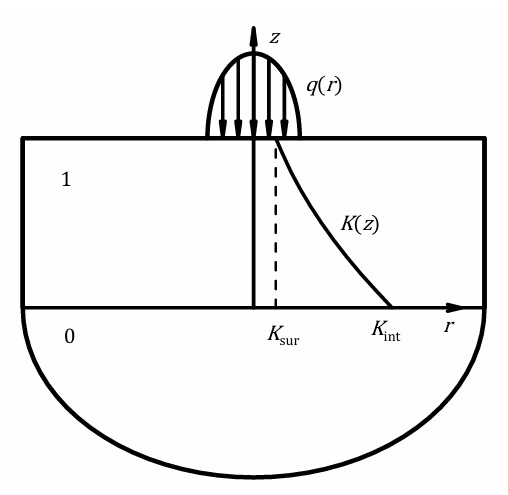
Suppose that the surface z =  = h of the graded coated half-space is heated by a heat flux of the graded coated half-space is heated by a heat flux q((r) = ) = q₀q^*((r) () (q^*(0) = 1) on the circle of radius (0) = 1) on the circle of radius a (Fig. 1); here (Fig. 1); here h =  = H//a, , H is the thickness of the coating, is the thickness of the coating, r and and z are dimensionless cylindrical coordinates referred to as normalized by the linear size are dimensionless cylindrical coordinates referred to as normalized by the linear size a. The remaining surface of the considered half-space is thermally insulated.. The remaining surface of the considered half-space is thermally insulated.

The half space consists of a homogeneous isotropic half-space with the heat conductivity coefficient K₀ and an gradient coating with the heat conductivity coefficient and an gradient coating with the heat conductivity coefficient K((z) = ) = K_intK^*((z) () (K^*(0) = 1), which can vary along its thickness. The perfect thermal contact between the coating and the substrate is assumed.(0) = 1), which can vary along its thickness. The perfect thermal contact between the coating and the substrate is assumed.

The dependence of the dimensionless heat conductivity coefficient K^* on the coordinate on the coordinate z is described by the formula: is described by the formula:

where the parameters K_int, , α and and β are known. are known.

The analysed problem is reduced to the solution of the following boundary problem:

equations:

Boundary conditions

where T_C and and T_S are the dimensionless temperature in the coating and substrate respectively; dimensionless temperature is related to the parameter are the dimensionless temperature in the coating and substrate respectively; dimensionless temperature is related to the parameter q₀a//K_sur; ; K_sur is the heat conduction coefficient on the surface of the considered inhomogeneous half-space; is the heat conduction coefficient on the surface of the considered inhomogeneous half-space; H((r) is Heaviside step function.) is Heaviside step function.

ANALYTICAL METHOD OF SOLUTION

The general solution of the differential equations (2) is sought by applying the Hankel integral transformation [26]:

where J₀ is the Bessel function. is the Bessel function.

The Hankel transform of the temperature for the substrate that satisfies the regularity conditions at infinity (5) can be written in the form:

where t₀((s) is the unknown function.) is the unknown function.

Applying the technique of the Hankel integral transformation to the partial differential equation (2a), the ordinary linear differential equation with variable coefficients is obtained:

The analytical form of the solution of the equation (8) is known only for selected forms of the function K^*((z). If the function ). If the function K^*((z) is described by formula (1), the general solution has the form [27]) is described by formula (1), the general solution has the form [27]

where t₁((s) and ) and t₂((s) are the unknown functions, ) are the unknown functions, ζ = 1 +  = 1 + αz, , p = 0.5(1 –  = 0.5(1 – β), ), I_p and and K_p are the modified Bessel’s functions. are the modified Bessel’s functions.

Satisfying boundary conditions (3) and (4), the functions t_i((s), ), i = 0, 1, 2 are obtained from solving a system of three linear equations: = 0, 1, 2 are obtained from solving a system of three linear equations:

where

q‾*(s) is Hankel transform of function is Hankel transform of function q^*((r))H(1 – (1 – r), ), ζ_h = 1 +  = 1 + αh..

To calculate the temperature in the physical domain, the inverse transformation is used:

As shown by previous studies, the most difficult integrals to calculate are obtained when calculating the temperature and heat flux in the radial direction on the surface of the considered inhomogeneous half-space:

where

The integral (13) is computed with regard for the asymptotic behavior of the function TC*(s) as as s → ∞: → ∞:

It should be noted that by replacing in the integrals (13) the function TC*(s) with its asymptote (15), we obtain formulas for calculating the temperature with its asymptote (15), we obtain formulas for calculating the temperature T_hom and heat flux in the radial direction and heat flux in the radial direction q_hom on the surface of a homogeneous half-space with the heat conductivity coefficient on the surface of a homogeneous half-space with the heat conductivity coefficient K_sur..

The integrals, in which the function TC*(s) is replaced by the asymptote (15), are calculated analytically. The remaining integrals are computed by using the Gaussian quadrature. is replaced by the asymptote (15), are calculated analytically. The remaining integrals are computed by using the Gaussian quadrature.

In particular, when

formulas for calculating the state functions on the surface of the homogeneous half-space have form

where F is hypergeometric function. is hypergeometric function.

REPLACING THE INHOMOGENEOUS COATING WITH A LAYER PACKAGE

In cases where the analytical solution of the differential equation (8) is not known, the inhomogeneous coating is replaced by a multilayer system of n homogeneous or inhomogeneous layers (Fig. 2).

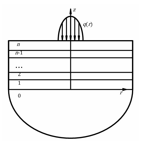
The layer with the number i ( (i =1, …,  =1, …, n) occupies the region 0 ≤ ) occupies the region 0 ≤ r <∞,  <∞, h_i-1 ≤  ≤ z  ≤   ≤ h_i ( (h₀ = 0,  = 0, h_n =  = h), and its thermal properties are described by the thermal conductivity coefficient ), and its thermal properties are described by the thermal conductivity coefficient K_i((z), which can vary along the thickness of the layer. After performing the Hankel integral transformation in each coating layer, the equation with the structure (8) is solved. A necessary condition for applying this approach is the existence of an analytical solution defined in the layer under consideration, which can be written as:), which can vary along the thickness of the layer. After performing the Hankel integral transformation in each coating layer, the equation with the structure (8) is solved. A necessary condition for applying this approach is the existence of an analytical solution defined in the layer under consideration, which can be written as:

where index i is the layer number in the considered package, is the layer number in the considered package, i = 1, 2, …,  = 1, 2, …, n, functions , functions f_k((s,,z), ), k = 1, …, 2 = 1, …, 2n are known fundamental solutions, functions are known fundamental solutions, functions t_k((s), ), k = 1, …, 2 = 1, …, 2n are unknown functions of the integral transform parameter. are unknown functions of the integral transform parameter.

In the framework of the problem under consideration, this condition is satisfied when the thermal conductivity coefficient of the layer is constant (approach A1) or its change along the layer thickness is described by a linear function (approach A2) or an exponential function (approach A3).

If the heat conduction coefficient of the layer with the number i is constant and equal to the means value of the function is constant and equal to the means value of the function K((z) in the region () in the region (h_i-1, , h_i):):

fundamental solutions f_2i-1((s,,z) and ) and f_2i((s,,z) can be written in the form:) can be written in the form:

If the heat conduction coefficient of the layer with the number i is described by linear function is described by linear function K_i((z) = ) = k_i(1+(1+β_iz) or exponential function ) or exponential function K_i((z) = ) = k_iexp(exp(β_iz), the parameters ), the parameters k_i and and β_i are calculated based on equations: are calculated based on equations: K_i((h_i-1) = ) = K((h_i-1), ), K_i((h_i) = ) = K((h_i).).

In the A2 approach, the fundamental solutions f_2i-1((s,,z) and ) and f_2i((s,,z) are as follows:) are as follows:

In the A3 approach, the fundamental solutions f_2i-1((s,,z) and ) and f_2i((s,,z) can be written in the form:) can be written in the form:

where γi=12βi2+4s2, , h̆i=hi−z.

An important feature of the fundamental solutions written in approaches A1 and A3 by formulas (20) and (22), respectively, is that the largest value of the argument of hyperbolic functions is equal to s((h_i -  - h_i-1) (approach A1) or ) (approach A1) or γ_i((h_i -  - h_i-1) (approach A3). Given that ) (approach A3). Given that h_i -  - h_i-1 << 1, succeeds in calculating the values of hyperbolic functions for large values of the parameter  << 1, succeeds in calculating the values of hyperbolic functions for large values of the parameter s..

The solution in the substrate is still defined by formula (7). The unknown functions t_k(s), (s), k = 0, 1, …, 2 = 0, 1, …, 2n are determined from the boundary conditions (3), (4) and the conditions of ideal thermal contact at the surfaces separating the coating layers. Once these conditions are satisfied, a system of 2 are determined from the boundary conditions (3), (4) and the conditions of ideal thermal contact at the surfaces separating the coating layers. Once these conditions are satisfied, a system of 2n + 1 algebraic linear equations depending on the parameter  + 1 algebraic linear equations depending on the parameter s is obtained: is obtained:

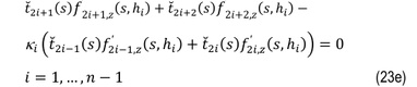
where

fk,z’,k=1,…,2n is the derivative of the function is the derivative of the function f_k((z) with respect to the variable ) with respect to the variable z, , κ₀ =  = K₀//K_int, , κ_i =  = K_i//K_i+1, (approach A1), , (approach A1), κ_i = 1 (approach A2 and A3),  = 1 (approach A2 and A3), i = 1, …,  = 1, …, n – 1.– 1.

Formulas for calculating temperature and heat flux in the radial direction on the surface of the considered inhomogeneous half-space can be written in the form (13), where:

where s*=s(1+βnh)βn..

As in Chapter 3, in each of the considered approaches to solving the problem, the function TC*(s) tends to 1 when as tends to 1 when as s → ∞. → ∞.

SELECTED DIRECT NUMERICAL METHODS IN THE HANKEL TRANSFORM DOMAIN

The approaches considered in this chapter are again based on the use of the Hankel integral transformation. The solution in the substrate is still described by equation (7). The ordinary differential equation with variable coefficients (8) is solved numerically. One traditional approach to solving it (approach B1) is to divide the interval [0, h] into ] into N equal parts, and then replace the differential operator defining the differential equation (8) with a differential formula at each interior node. It can be shown [24] that: equal parts, and then replace the differential operator defining the differential equation (8) with a differential formula at each interior node. It can be shown [24] that:

In addition, using the form of equation (8), it can be proven that:

In the formulas (26) and (27), the designations have been introduced: hi*=ihN , T‾i=T‾Cz=hi*,i=0,1,…,N,Kl*=K*(lhN), l=i,i±12,i=1,…,N,Δz=hN . .

The use of differential formulas (26) and (27) makes it possible to reduce the solution of the problem under consideration to the solution of a system of N + 1 algebraic linear equations: + 1 algebraic linear equations:

and an additional linear equation:

In equations (28), the designations have been introduced:

The system of algebraic linear equations (28) is a tridiagonal matrix system. It is easy to see that the conditions for the stability of the Thomas algorithm are met [28], allowing it to be solved quickly and efficiently.

The solution to the system of equations can be written in the form:

where the parameters ϖ_i1 and and ϖ_i2, , i = 0, 1, …,  = 0, 1, …, N, are the solutions of the system of equations with the matrix of the system of equations (28) and the free terms described by the formulas, are the solutions of the system of equations with the matrix of the system of equations (28) and the free terms described by the formulas

δ_i0 and and δ_iN are Croneckere's symbols are Croneckere's symbols

Ultimately, functions T‾i(s),i=0,1,…,N and function and function t₀((s) can be determined using formulas:) can be determined using formulas:

Formulas for calculating temperature and heat flux in the radial direction on the surface of the considered inhomogeneous half-space can be written in the form (13), where:

It can be shown that the function sTC*(s) tends to 0.5 tends to 0.5N//h when as when as s → ∞. → ∞.

An alternative approach B2 to numerically solving the differential equation (8) is to construct its solution in the form

It is easy to see that:

The equation (8) will be satisfied when

The boundary conditions (4) will be satisfied when

As it follows from equations (36) and (37), the functions A_T((s, , z) and ) and A_Q((s, , z) are the solution of the Cauchy problem for a system of two ordinary differential equations. After numerically solving this problem using the Runge-Kutta method, the function ) are the solution of the Cauchy problem for a system of two ordinary differential equations. After numerically solving this problem using the Runge-Kutta method, the function t₀((s) is calculated from the formula) is calculated from the formula

In the process of using the Runge-Kutta method, the interval [0, h] is divided into ] is divided into N subintervals, and then for the given value of the parameter subintervals, and then for the given value of the parameter s the values the values A_T((s, , z_i) and ) and A_Q((s, , z_i), ), i = 1, 2, …,  = 1, 2, …, N are calculated. The main advantage is that the calculation process is iterative. The values are calculated. The main advantage is that the calculation process is iterative. The values A_T((s,,z_i) and ) and A_Q((s, , z_i) in the node with number ) in the node with number i are calculated according to the adopted Runge-Kutta scheme using only the values are calculated according to the adopted Runge-Kutta scheme using only the values A_T((s, , z_i-1) and ) and A_Q((s, , z_i-1) in the previous node. Traditionally, it is assumed that the scheme has the accuracy O(() in the previous node. Traditionally, it is assumed that the scheme has the accuracy O((h//N))⁴).).

Similarly as before, the temperature and heat flux in the radial direction on the surface of the considered inhomogeneous half-space are calculated from the formula (13) in which:

Calculations show that the function TC*(s) described by the formula (39) tends to 1 when as described by the formula (39) tends to 1 when as s → ∞. → ∞.

NUMERICAL EXAMPLES AND DISCUSSION

We assume that the heat flux q^*((r) is described by formula (16). In order to compare the analytical solution described by the formulas (13) and (14) with the approximate solution obtained using the numerical approaches considered, we will believe that the parameter ) is described by formula (16). In order to compare the analytical solution described by the formulas (13) and (14) with the approximate solution obtained using the numerical approaches considered, we will believe that the parameter β determining the dependence of the dimensionless heat conductivity coefficient determining the dependence of the dimensionless heat conductivity coefficient K^* on the on the z-coordinate in formula (1) is equal to 2. In addition, we accept that -coordinate in formula (1) is equal to 2. In addition, we accept that h = 0.5,  = 0.5, K_int =  = K₀, , K_int = 5 = 5K_sur or or K_int = 10 = 10K_sur, i.e., the thermal conductivity coefficient at the interface between the coating and the substrate is continuous, and the considered gradient coating is a thermal insulator., i.e., the thermal conductivity coefficient at the interface between the coating and the substrate is continuous, and the considered gradient coating is a thermal insulator.

Under such assumptions, the parameter α is calculated from the formula: is calculated from the formula:

If an approximate solution is constructed using approach A1, the thermal conductivity coefficients of homogeneous layers are equal to:

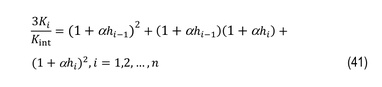
In the A2 approach, the parameters β_i and and k_i describing the change in the thermal conductivity coefficient along the layer thickness are calculated based on the formulas: describing the change in the thermal conductivity coefficient along the layer thickness are calculated based on the formulas:

The corresponding formulas in the A3 approach are:

Previous studies of similar problems show [21, 23] that the greatest differences between analytical and numerical solutions are to be expected when calculating the state function on the surface of the considered inhomogeneous half-space. Given that the function q_r((r, , h) has no derivative at the edge of the heating area, its calculation at this point is particularly challenging. Therefore, we will focus on calculating the value of ) has no derivative at the edge of the heating area, its calculation at this point is particularly challenging. Therefore, we will focus on calculating the value of q_r(1, (1, h) and the value of the maximum dimensionless temperature, that is, the temperature ) and the value of the maximum dimensionless temperature, that is, the temperature T_C(0, (0, h). To calculate the marked values, you need to calculate the integrals ). To calculate the marked values, you need to calculate the integrals IT∞=TC(0,h) and and Iq∞=q0-1q(1,h) described by formulas (13). When calculating improper integrals of the first kind, we replace them with integrals described by formulas (13). When calculating improper integrals of the first kind, we replace them with integrals ITS and and IqS, where the number , where the number S is the upper limit of integration. To reduce the effect of the accuracy of calculating the integrals on the accuracy of the obtained solutions, we choose the value of the parameter is the upper limit of integration. To reduce the effect of the accuracy of calculating the integrals on the accuracy of the obtained solutions, we choose the value of the parameter S so that so that

where ε is the permissible error in calculating the integral is the permissible error in calculating the integral I_q..

However, it should be noted that a characteristic feature of the considered approaches is that for relatively large values of the parameter S there is a loss of stability of the calculation, which makes it impossible in some cases to meet the criterion introduced. there is a loss of stability of the calculation, which makes it impossible in some cases to meet the criterion introduced.

In evaluating the effectiveness of the analytical-numerical approaches under consideration, we will assess three aspects: 1) the accuracy of calculating the temperature at the center of the heating zone and the heat flux in the radial direction at the edge of the heating zone obtained for the given value of the parameter n (approaches A) or (approaches A) or N (approaches B); 2) the range of the parameter (approaches B); 2) the range of the parameter s necessary to calculate with satisfactory accuracy the integrals described by equation (13) and the stability of calculating the function necessary to calculate with satisfactory accuracy the integrals described by equation (13) and the stability of calculating the function TC*(s) for relatively large values of the parameter for relatively large values of the parameter s, 3) a comparison of the time costs necessary to obtain satisfactory accuracy of the approximate solution., 3) a comparison of the time costs necessary to obtain satisfactory accuracy of the approximate solution.

The values of T_C(0, (0, h) and ) and q_r(1, (1, h)/)/q₀ obtained from the analytical solution for two values of the parameter obtained from the analytical solution for two values of the parameter K₀//K_sur are presented in the corresponding columns of Tables 1 and 2. To compare the differences between the solutions, which are caused by the use of analytical-numerical approaches A1, A2 and A3 to solve the problem, in the rows with are presented in the corresponding columns of Tables 1 and 2. To compare the differences between the solutions, which are caused by the use of analytical-numerical approaches A1, A2 and A3 to solve the problem, in the rows with n = 160, 80, 40, 20, and 10 (Table 1, approach A1) and the rows with  = 160, 80, 40, 20, and 10 (Table 1, approach A1) and the rows with n = 80,40, 20, and 10 (Table 2, approaches A2 and A3) the relative deviations (given in percent) obtained for the multilayer coating with the indicated number of layers are presented. The values in these rows were obtained for the value of the parameter  = 80,40, 20, and 10 (Table 2, approaches A2 and A3) the relative deviations (given in percent) obtained for the multilayer coating with the indicated number of layers are presented. The values in these rows were obtained for the value of the parameter S, satisfying the condition (44), in which the , satisfying the condition (44), in which the ε = 10 = 10^-5 (approaches A1 and A3); (approaches A1 and A3);ε = 2.5⋅10 = 2.5⋅10^-5 (approach A2). The column of Table 1 marked with the symbol (approach A2). The column of Table 1 marked with the symbol S lists the values of parameter lists the values of parameter S for which condition (44) has been satisfied. for which condition (44) has been satisfied.

The values of T_C(0, (0, h) and ) and q_r(1, (1, h)/)/q₀ obtained from the analytical solution for two values of the parameter obtained from the analytical solution for two values of the parameter K₀//K_sur are presented in the corresponding columns of Tables 1 and 2. To compare the differences between the solutions, which are caused by the use of analytical-numerical approaches A1, A2 and A3 to solve the problem, in the rows with are presented in the corresponding columns of Tables 1 and 2. To compare the differences between the solutions, which are caused by the use of analytical-numerical approaches A1, A2 and A3 to solve the problem, in the rows with n = 160, 80, 40, 20, and 10 (Table 1, approach A1) and the rows with  = 160, 80, 40, 20, and 10 (Table 1, approach A1) and the rows with n = 80,40, 20, and 10 (Table 2, approaches A2 and A3) the relative deviations (given in percent) obtained for the multilayer coating with the indicated number of layers are presented. The values in these rows were obtained for the value of the parameter  = 80,40, 20, and 10 (Table 2, approaches A2 and A3) the relative deviations (given in percent) obtained for the multilayer coating with the indicated number of layers are presented. The values in these rows were obtained for the value of the parameter S, satisfying the condition (44), in which the , satisfying the condition (44), in which the ε = 10 = 10^-5 (approaches A1 and A3); (approaches A1 and A3);ε = 2.5⋅10 = 2.5⋅10^-5 (approach A2). The column of Table 1 marked with the symbol (approach A2). The column of Table 1 marked with the symbol S lists the values of parameter lists the values of parameter S for which condition (44) has been satisfied. for which condition (44) has been satisfied.

As can be seen from Tables 1 and 2, all three proposed approaches A allow for fairly accurate temperature calculations. However, the heat flux at the edge of the heating zone with satisfactory accuracy for a relatively small number of layers in the package is obtained only in approaches A2 and A3. The results obtained in these approaches are similar with the difference that the deviations from the analytical solution have opposite signs. In approach A1, an error in the heat flux calculation q_r(1, (1, h) of about 1% is obtained when ) of about 1% is obtained when n = 160. It should be noted that in approach A1 such large errors in the heat flux calculation are observed only in the relatively small vicinity of the heating zone edge. = 160. It should be noted that in approach A1 such large errors in the heat flux calculation are observed only in the relatively small vicinity of the heating zone edge.

In all approaches, doubling the number of layers in the package results in a four-fold reduction in the difference between the analyzed temperature values. At the same time, in approach A1, a two-fold reduction in the difference between the analyzed heat flux values is observed, and in approaches A2 and A3, a four-fold reduction. This trend is distorted by an error made in the calculation of integral (13). Because the error in the calculation of the integral does not depend on the number of layers in the package, this distortion is more pronounced for larger values of parameter n, for which a smaller difference between the analytical and numerical solutions is obtained., for which a smaller difference between the analytical and numerical solutions is obtained.

Analysis of the system of equations (23) shows that in approaches A1, A2 and A3 the determinant of the matrix of the system of equations approaches zero when the parameter s approaches infinity. This means that there is a critical value of the parameter approaches infinity. This means that there is a critical value of the parameter s, beyond which the calculations lose stability. At the same time, it can be observed that, compared to approach A1, in approaches A2 and A3 the function , beyond which the calculations lose stability. At the same time, it can be observed that, compared to approach A1, in approaches A2 and A3 the function TC*(s) approaches its asymptotic value more slowly for large values of the parameter approaches its asymptotic value more slowly for large values of the parameter s. As a result, in approaches A2 and A3 the critical value of the parameter . As a result, in approaches A2 and A3 the critical value of the parameter s is larger than the corresponding value in approach A1. For parameter is larger than the corresponding value in approach A1. For parameter ε = 10 = 10^-5 in approach A3 this value ranged from 2800 ( in approach A3 this value ranged from 2800 (K₀//K_sur = 10) to 3200 ( = 10) to 3200 (K₀//K_sur = 5). = 5).

An important advantage of approaches A1 and A3 over approach A2 is a certain freedom in choosing the form of fundamental solutions. The special choice of these forms, described by formulas (20) and (22), allows us to obtain for a selected large value of the parameter s a relatively small value of the argument of the functions describing the fundamental solutions. This allows us to expand the range of the parameter a relatively small value of the argument of the functions describing the fundamental solutions. This allows us to expand the range of the parameter s in which the calculations are stable. The range is so wide that condition (44) could be fulfilled even for a parameter in which the calculations are stable. The range is so wide that condition (44) could be fulfilled even for a parameter ε value that is several tens of times less than 10 value that is several tens of times less than 10^-5. In approach A2, the solutions are described by special functions whose form does not allow this to be done. As a result, in approach A2, the critical value of the parameter . In approach A2, the solutions are described by special functions whose form does not allow this to be done. As a result, in approach A2, the critical value of the parameter s for the considered values of the parameters for the considered values of the parameters h and and K₀//K_sur is approximately 1500 ( is approximately 1500 (K₀//K_sur = 5) or approximately 1800 ( = 5) or approximately 1800 (K₀//K_sur = 10), which makes it impossible to fulfill condition (44) for the parameter  = 10), which makes it impossible to fulfill condition (44) for the parameter ε = 10 = 10^-5. Condition (44) would be fulfilled when the permissible error in calculating the integral . Condition (44) would be fulfilled when the permissible error in calculating the integral I_q would be taken at the level of would be taken at the level of ε = 2.5⋅10 = 2.5⋅10^-5..

Accepting a larger error in the calculation of integral (13) does not always result in a larger difference between the analytical and numerical solutions. Sometimes the error in calculating the integral and the error in the numerical method have opposite signs. In such a case, reducing the value of parameter S within a certain range will even improve the obtained numerical solution. We observe this in the problem under consideration. However, such a conclusion can only be valid when the analytical solution is known. Because the numerical approach is used when such a solution is unknown, the discussed feature of approach A2 is disadvantageous. It should be noted that in approach A2, the critical value of parameter within a certain range will even improve the obtained numerical solution. We observe this in the problem under consideration. However, such a conclusion can only be valid when the analytical solution is known. Because the numerical approach is used when such a solution is unknown, the discussed feature of approach A2 is disadvantageous. It should be noted that in approach A2, the critical value of parameter s decreases as the values of parameters decreases as the values of parameters h or or K_sur//K₀ increase. Therefore, applying approach A2 for thicker coatings may be ineffective. increase. Therefore, applying approach A2 for thicker coatings may be ineffective.

A significant drawback of the numerical approaches described in Chapter 4 is that, when calculating the integrals described by formula (13), for each value of the parameter s taken from a given set of parameters, one must solve a system of linear algebraic equations of relatively large dimension 2 taken from a given set of parameters, one must solve a system of linear algebraic equations of relatively large dimension 2n + 1. The matrix structure of this system is such that it is difficult to propose a fast algorithm for its solution. The classical Gaussian elimination algorithm with principal element selection is used, which is quite time-consuming. An alternative is to use the difference method (approach B1) described in Chapter 5. This approach also yields a system of linear equations of dimension  + 1. The matrix structure of this system is such that it is difficult to propose a fast algorithm for its solution. The classical Gaussian elimination algorithm with principal element selection is used, which is quite time-consuming. An alternative is to use the difference method (approach B1) described in Chapter 5. This approach also yields a system of linear equations of dimension N + 1. However, this time, the stability of the Tomass algorithm can be proven [28] for the same number of equations, it is much faster than the Gauss algorithm. + 1. However, this time, the stability of the Tomass algorithm can be proven [28] for the same number of equations, it is much faster than the Gauss algorithm.

The results of the comparison of the analytical solution with the numerical solution obtained using approach B1 are presented in Table 3. The structure of this table is the same as that of Table 1. As can be seen from Table 3, satisfying condition (44) requires considering an integration interval that is much wider than the previously considered integration intervals. This requires solving the system of equations for a significantly larger number of parameters s. However, the Tomass algorithm is fast enough to be considered with 641 nodes (. However, the Tomass algorithm is fast enough to be considered with 641 nodes (N = 640), and this is not the limit of its capabilities. It is also important that no loss of stability of the calculations was observed for large values of parameter  = 640), and this is not the limit of its capabilities. It is also important that no loss of stability of the calculations was observed for large values of parameter s. This means that using approach B1, the time costs of calculating the temperature with the accuracy presented in Tables 1 and 2 are much lower than similar costs in the previously considered approaches.. This means that using approach B1, the time costs of calculating the temperature with the accuracy presented in Tables 1 and 2 are much lower than similar costs in the previously considered approaches.

The calculations show that approach B1 is also effective for calculating heat fluxes, with the exception of calculating the flux in the relatively small vicinity of the heating region's edge. At the same time, a relatively large error in calculating the flux q_r(1, (1, h) is observed. In problems where the accuracy of calculating the value of the state function ) is observed. In problems where the accuracy of calculating the value of the state function q_r(1, (1, h) or similar state functions in other problems is important, approach B1 should be considered inefficient.) or similar state functions in other problems is important, approach B1 should be considered inefficient.

Approach B2 is an approach whose speed of obtaining results is commensurate with the speed of approach B1. A drawback of the method is the possibility of loss of stability of the calculations if the parameter N is incorrectly selected. Calculations have shown that as the parameter is incorrectly selected. Calculations have shown that as the parameter s increases, for which the iterative Runge-Kutta scheme is performed, the value of parameter increases, for which the iterative Runge-Kutta scheme is performed, the value of parameter N should be increased. The calculations will be stable when a proper relationship between the parameters should be increased. The calculations will be stable when a proper relationship between the parameters N and and s is chosen, for example the relationship: is chosen, for example the relationship:

where N₀ ≥ 10 – value of parameter  ≥ 10 – value of parameter N for relatively small values of parameter for relatively small values of parameter s..

The results of the comparison of the analytical solution with the numerical solution obtained using the B2 approach are presented in Table 4, the structure of which is the same as in Tables 1 or 3.

CONCLUSIONS

The aim of this paper is to present five analytical-numerical algorithms that allow for the construction of approximate solutions to problems for the gradient coating with continuous change of properties along the coating thickness. The comparison of the proposed approaches was performed using the axisymmetric heat conduction problem describing the local heating of the half-space surface with the gradient coating. It was assumed that the change in the thermal conductivity coefficient along the coating thickness is described by parabolic function K(z) =  = K_int(1+αz)². The choice of this function was based on the possibility of obtaining an analytical solution.. The choice of this function was based on the possibility of obtaining an analytical solution.

The analytical part of the considered approaches in all proposed algorithms was based on the Hankel integral transform. The boundary value problem for partial differential equations defined in the coating and substrate was reduced to the boundary value problem for ordinary differential equations. The resulting problem depended on the integral transform parameter s. After obtaining its approximate solution, an inverse integral transform was performed, consisting in calculating improper integrals of the first kind (12), and in particular integrals (13) describing the temperature at the center of the heating zone and the radial heat flux at the edge of the heating zone.. After obtaining its approximate solution, an inverse integral transform was performed, consisting in calculating improper integrals of the first kind (12), and in particular integrals (13) describing the temperature at the center of the heating zone and the radial heat flux at the edge of the heating zone.

Two methods were proposed to construct the approximate solution to the obtained boundary value problem. The first method, designated A, consisted of replacing the coating with the continuously varying thermal conductivity coefficient with the multilayer coating. In approach A1, homogeneous layers were considered. The thermal conductivity coefficient of each layer was obtained by calculating the average value of the K((z) function over the range of the considered layer. In approaches A2 and A3, the layers were inhomogeneous. The change in thermal conductivity coefficient along the layer thickness was described by the linear function (approach A2) or the exponential function (approach A3). These functions contained two unknown parameters, which were determined by interpolation. In all approaches described in Chapter 4, the analytical solution was constructed in each layer of the package, and then the boundary value problem was reduced to solving the system of linear equations of dimension 2) function over the range of the considered layer. In approaches A2 and A3, the layers were inhomogeneous. The change in thermal conductivity coefficient along the layer thickness was described by the linear function (approach A2) or the exponential function (approach A3). These functions contained two unknown parameters, which were determined by interpolation. In all approaches described in Chapter 4, the analytical solution was constructed in each layer of the package, and then the boundary value problem was reduced to solving the system of linear equations of dimension 2n + 1, solved by the Gaussian method with principal element selection. + 1, solved by the Gaussian method with principal element selection.

Comparison of the approximate solutions obtained by method A with the exact solution showed that the error in calculating the maximum temperature did not exceed 0.2%, even with a relatively small number of layers (n = 20). When calculating the heat flux  = 20). When calculating the heat flux q_r(1, (1, h), an error of this level at ), an error of this level at n = 20 was obtained only in approaches A2 and A3. In approach A1, even when 160 layers were considered, the error in flux  = 20 was obtained only in approaches A2 and A3. In approach A1, even when 160 layers were considered, the error in flux q_r(1, (1, h) calculation was approximately 1%. Although in this approach such large errors in the calculation of the heat flux ) calculation was approximately 1%. Although in this approach such large errors in the calculation of the heat flux q_r(1, (1, h) were observed only in the relatively small vicinity of the edge of the heating area, the highlighted shortcoming may be the basis for rejecting approach A1. It should be noted that in the theory of elasticity [21] or thermoelasticity [23] the analog of the state function ) were observed only in the relatively small vicinity of the edge of the heating area, the highlighted shortcoming may be the basis for rejecting approach A1. It should be noted that in the theory of elasticity [21] or thermoelasticity [23] the analog of the state function q_r((r,, z) is the radial stress ) is the radial stress σ_rr, whose value at point (1, , whose value at point (1, h) often determines the highest tensile stress. Therefore, calculating the derivatives of the state function at the boundary of the area of influence of the external factor may be of fundamental importance.) often determines the highest tensile stress. Therefore, calculating the derivatives of the state function at the boundary of the area of influence of the external factor may be of fundamental importance.

When comparing approaches A2 and A3, it should be noted that when parameter s exceeds a certain critical value, the calculations lose stability. However, in approach A3, the range of parameter exceeds a certain critical value, the calculations lose stability. However, in approach A3, the range of parameter s over which the calculations are stable is more than ten times wider than the corresponding range in approach A2. This is achieved through a special selection of functions describing the analytical solutions in the layers of the package. The argument of these functions is not the global coordinate over which the calculations are stable is more than ten times wider than the corresponding range in approach A2. This is achieved through a special selection of functions describing the analytical solutions in the layers of the package. The argument of these functions is not the global coordinate z, but the local coordinate , but the local coordinate h_i –  – z, which is assigned to the top surface of the layer. The result of this choice is that, within the layer thickness range, the argument , which is assigned to the top surface of the layer. The result of this choice is that, within the layer thickness range, the argument h_i – – z takes much smaller values than the argument takes much smaller values than the argument z. In approach A2, the fundamental solutions are described by special functions [8, 9, 13, 14], which causes a certain rigidity in the choice of the form of the fundamental solutions.. In approach A2, the fundamental solutions are described by special functions [8, 9, 13, 14], which causes a certain rigidity in the choice of the form of the fundamental solutions.

The main drawback of the preferred A3 approach, as well as the A2 approach, is that their applicability depends on the ability to construct an analytical solution within the layers of the package. It is known [21] that in the case of the A3 approach, such a possibility occurs in three-dimensional problems of the theory of elasticity for an isotropic layer with a constant Poisson's ratio. In the case of thermoelasticity problems or problems of the theory of elasticity for a transversely isotropic layer, the ability to obtain an analytical solution is conditioned by additional relationships between parameters describing the material properties. The class of problems to which the A2 algorithm can be applied is even narrower.

In terms of the ability to construct an analytical solutions within the layers of the package, the A1 approach is the most universal. This capability exists in all the aforementioned problems of elasticity or thermoelasticity theory. This is likely the fundamental reason for the widespread use of this algorithm to solve a variety of problems [18-21, 23].

Using the A1, A2, or A3 approaches to solving problems for the gradient coating with continuously varying properties, which arise when modelling multilayer coatings described by homogenization methods [29–31] raises an additional dissatisfaction: one multilayer coating is replaced by another multilayer coating. Therefore, another method, designated as B, was proposed, which involves numerically solving boundary value problems arising in the space of transform.

For this purpose, difference formulas [24] are often used to approximate differential operators (approach B1). This approach again yields a system of linear equations of dimension N + 1. Studies have shown that the B1 approach can be advantageous over approaches A1, A2, or A3 only when the matrix of the system is a tridiagonal matrix, for which the stability conditions of the Tomass algorithm are proven. Then, the time cost of solving the system of equations is much lower. The second important condition is the use of difference formulas that approximate the differential operators appearing in the boundary value problem with an accuracy no lower than  + 1. Studies have shown that the B1 approach can be advantageous over approaches A1, A2, or A3 only when the matrix of the system is a tridiagonal matrix, for which the stability conditions of the Tomass algorithm are proven. Then, the time cost of solving the system of equations is much lower. The second important condition is the use of difference formulas that approximate the differential operators appearing in the boundary value problem with an accuracy no lower than Δz2. If the differential equation is described by the differential operator . If the differential equation is described by the differential operator Lf = ( = (K((z))f ′(′(z))′, such a possibility exists [24]. It was presented in the first part of Chapter 5.))′, such a possibility exists [24]. It was presented in the first part of Chapter 5.

The accuracy of temperature calculations using the B1 approach is comparable to that of previous approaches. Good accuracy is also obtained when calculating the heat flux q_r((r, , z) over the entire coverage, except for a certain area surrounding the edge of the heating region. If calculations in this area are not essential, then, given the low computational time costs, the B1 method can be considered an advantage over methods A1, A2, and A3. Unfortunately, the low accuracy of calculating the flux ) over the entire coverage, except for a certain area surrounding the edge of the heating region. If calculations in this area are not essential, then, given the low computational time costs, the B1 method can be considered an advantage over methods A1, A2, and A3. Unfortunately, the low accuracy of calculating the flux q_r(1, (1, h) may be grounds for rejecting this method. The second major drawback is the relatively limited applicability of the B1 approach, due to the need to meet the two important conditions described above. In addition to heat conduction problems, the method can most likely be applied to torsion problems similar to the problem [17].) may be grounds for rejecting this method. The second major drawback is the relatively limited applicability of the B1 approach, due to the need to meet the two important conditions described above. In addition to heat conduction problems, the method can most likely be applied to torsion problems similar to the problem [17].

An alternative method for numerically solving the boundary value problem is the B2 algorithm. Unlike other approaches, the B2 approach does not reduce to solving linear algebraic equations. In the B2 method, which should be considered very original, the boundary value problem is reduced to the Cauchy problem for a system of two ordinary differential equations. The speed of this method is comparable to the speed of the B1 method, and the accuracy of calculating the T_C(0, (0, h) and ) and q_r(1, (1, h) values is comparable to the accuracy of the A3 method. A drawback of B2 method is the possibility of loss of calculation stability if the relationship between the method parameter ) values is comparable to the accuracy of the A3 method. A drawback of B2 method is the possibility of loss of calculation stability if the relationship between the method parameter N and the integral transformation parameter and the integral transformation parameter s is incorrectly chosen. Calculations have shown that in the problem under consideration, the value of parameter is incorrectly chosen. Calculations have shown that in the problem under consideration, the value of parameter N should increase with increasing parameter should increase with increasing parameter s..

The feasibility of using the B2 approach to solve problems in the theory of elasticity or thermoelasticity is not obvious and requires additional research. However, there is a high probability that this approach will be effectively applied not only to problems involving gradient isotropic coatings, but also to gradient transversely isotropic coatings.