INTRODUCTION

In engineering practice, thin films and thin-film elements have found widespread application [1-4]. In these elements, surface and bulk factors contribute comparably to their overall energy. Particles located on the surface of a body experience interactions only from the internal regions, whereas particles in the deeper layers of the body interact isotropically in all directions. This implies that the binding energy of a particle changes as one moves from the surface into the bulk of the material. Such inhomogeneity results in a nonzero stress-strain state, which is sometimes accounted for by incorporating surface energy effects into the model [5-9]. Properly accounting for near-surface inhomogeneity allows for the description of various size-dependent effects, including surface stresses and mechanical strength. The binding energy within a material is closely related to its mass density, and near-surface inhomogeneity can be linked to surface roughness. In a single-component solid body, variations in mass density inhomogeneity are typically correlated with changes in porosity.

Geometric inhomogeneity is an inherent characteristic of every real surface, regardless of its formation or processing method. To quantify surface roughness, various numerical parameters are used, distinguishing between the surface's three-dimensional description and its profile's two-dimensional representation. A key parameter in surface profiling is the bearing area curve, known as the Abbott-Firestone curve or material ratio curve. Originally developed to analyze the contact between two surfaces, this curve illustrates the relationship between the actual contact area and the separation distance of the surfaces [10, 11]. When a surface is depicted through a profilometric contour, the Abbott-Firestone curve, as a function of height z, represents the fraction of the nominal area contained within the surface contour at elevation z. In other words, it quantifies the percentage of space occupied by the material at a given height within the real surface profile.

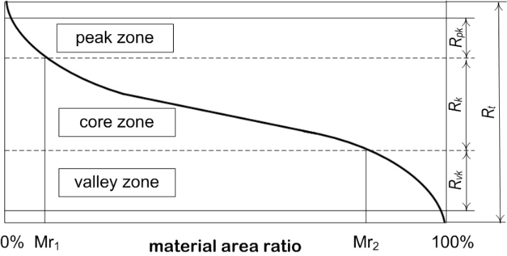
Figure 1 illustrates the key features of the curve along with the Rk family parameters. Here, Rt represents the total height of the roughness profile, defined as the distance between its highest peak and lowest valley. Rk represents the thickness of the core zone. The parameters Mr1 and Mr2 are percentage values that characterize the core zone, usually with Mr2=80% and Mr1=5% or 10%. Parameters Rpk and Rvk correspond to the average heights of the peaks above and the valleys below the core zone, respectively. Note, lower Rpk values indicate higher abrasion resistance and an increased contact area, whereas higher Rvk values suggest an improved capacity of the surface to retain lubricant.

The curve is typically used in manufacturing and quality control for tribology and wear analysis, as well as for evaluating lubrication performance [12, 13]. It is determined experimentally based on a profilometer scan of the surface, which generates a surface height profile. Its physical significance is related to the concept of mass density since the portion of space occupied by the material corresponds to the mass density of a porous material.

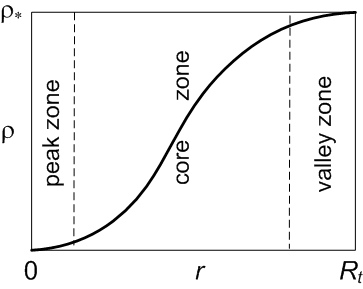
If the Abbott-Firestone curve is plotted as mass density ρ versus distance r measured from the highest point of the surface profile to the depth of the body, it will resemble the representation shown in Fig. 2. Here ρ* represents the mass density of a solid medium of the identical material. This means that the microinhomogeneities of a real body's surface are characterized by near-surface mass density inhomogeneity within a continuum description, where the surface of the body is modeled as a smooth geometric surface (e.g. a plane) passing through the highest peak of the actual surface. In classical solid mechanics, mass density is typically assumed to be constant throughout the entire body and for a given material, it does not vary from point to point.

Near-surface mass density inhomogeneity and the effects related to the inhomogeneity of binding energy can be addressed within the framework of the local-gradient approach in thermomechanics [14-16]. In the study [17], a mathematical model of a locally inhomogeneous elastic body considering surface roughness was proposed. One of the equations of this model is the equation for mass density. Its solution for a body with flat boundaries reflects the regularities of the bearing ratio curve.

Considering the variation in mass density from point to point, an accurate description must account for the corresponding change in material properties including elastic characteristics such as the moduli of elasticity. In porous solids, Young's modulus E and Poisson's ratio ν are often related to the porosity coefficient ϕ by the following relationships

Here, quantities intrinsic to the fully dense (non-porous) material (in the reference state) are denoted by an asterisk. These dependencies are widely reported in literature and are supported both experimentally [18-20] and theoretically, particularly through homogenization methods [21-23]. Since porosity reflects the amount of void space in a material, these relationships can also be expressed in terms of mass density:

This is especially important in thin films, where the size of the near-surface mass density inhomogeneity region can be comparable to the thickness of the body. It is also worth noting that, knowing the dependencies of Young's modulus and Poisson's ratio on density, one can, if necessary, derive similar relationships for other elastic moduli.

The objective of this work is to model and analyze how the surface roughness of a real body affects the elastic moduli in thin films. This study is conducted within the model of a locally inhomogeneous elastic body with surface roughness. In addition, it is investigated how the thickness of the near-surface region of mass density inhomogeneity, especially the regions of peaks and valleys, depends on the model parameters.

BASIC RELATIONS OF LOCAL GRADIENT APPROACH IN MECHANICS OF ELASTIC SOLIDS

One of the key equations of the locally inhomogeneous elastic body model is the equation for mass density [14, 17]

Here ξmis a parameter that characterizes the material structure of the body, dsm is a function accounting for the method of surface formation (referred to as mass sources for convenience), ∇2=∇→•∇→, where ∇→ is the del operator, and “•” stands for the dot product. It should be noted that mass sources allow us to consider the inhomogeneity of mass density in a region whose size differs significantly from the characteristic grain size of the material, which the parameter ξm is usually associated with [14]. When describing near-surface heterogeneity, it is reasonable to assume that the function dsm decreases to zero as it extends from the surface into the depth of the body.

In the paper [17], mass sources were proposed for bodies with nominally flat boundaries to account for the patterns of the bearing area curve. The parameters of these mass sources enable control over the size of near-surface heterogeneity regions, as well as the dimensions of peaks and valleys zones.

In the model of a locally inhomogeneous elastic body, the complete system of equations includes the equation (3) for mass density, along with the equations governing the elastic fields — specifically, those for the displacement vector and the stress or strain tensors.

The linearized equilibrium equation for the displacement vector u→ and mass density ρ takes the form

where amis a material parameter.

Choosing the stress tensor σ̂ as the solving function, instead of the displacement vector u→, results in another system of equations for the model. For this case, equation (4) should be replaced with the following two equations

Here σ=σ̂:Î, Î is the second order identity tensor, the symbols “:” and “×” denotes double inner and cross products respectively, the superscript T indicates transposition.

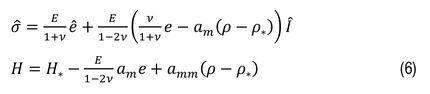
It is worth noting that the parameter conjugated to ρ is the thermodynamic chemical potential H, and the perturbation of the latter is associated with the perturbation of the binding energy [14, 15]. We also note that the stress tensor σ̂ and the thermodynamic chemical potential H are related to the strain tensor ê and the mass density ρ by the relations

and the strain tensor ê is related to the displacement vector u→ by the Cauchy relation

Here amm is a material parameter, H* is the thermodynamic chemical potential of the material in the reference state, e=ê:Î, ⨂ stands for the tensor product.

When formulating boundary value problems, the systems of equations (3), (4) or (3), (5) must be supplemented with an expression for dsm and the appropriate boundary conditions.

INTERFACE INHOMOGENEITY NEAR A NOMINALLY FLAT BOUNDARY

Let us consider an isotropic deformable half-space free from external force loading, occupying the domain x≥0 in the rectangular Cartesian coordinate system {x,y,z}. The reference state is taken to be the state of a homogeneous body, with constant mass density equal to ρ*. We assume that the surface of the body passes through the highest vertex of the profile of the real surface, therefore, we take the following boundary condition together with the condition of the mass density being bounded at infinity

The choice of the mass density at the surface of a body depends on various factors, including the modeling approach and the state of the surface. A method for justifying the determination of surface density is discussed in [24], which arrives at a value of ρ*/2 for a perfectly flat surface, with lower values for rougher surfaces. In general, the density at the surface of the solid can vary from 0 to ρ*. In this study, we rely on the Abbott-Firestone curve, which represents the percentage of space occupied by the material. We observe that at the boundary of the solid, this percentage starts from zero. Therefore, we assume that the density at the surface of the solid is zero.

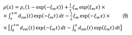
Assuming that dsm depends only on the coordinate x, the solution of equation (3), that satisfies conditions (8) can be written as:

In [17], the expression for the mass sources dsm was adopted as follows

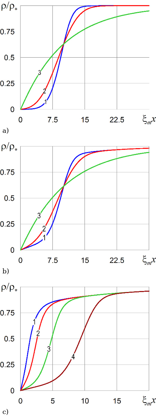
where a,b,k,ξs,ξsd are constant parameters. It is also shown that this representation allows considering the regularities of the material ratio curve into the mass density distribution, including the existence of peak, core and valley zones. This is illustrated in particular by the graphs in Fig. 3 which present the dependence of ρρ* on ξmx. In Fig. 3 a) a=1, ξsξm=0.1, k=6,3,1 (blue, red and green curves); in Fig. 3 b) a=0.8, ξsdξm=0.08, ξsξm=0.1, k=6,3,1 (curves 1–3); in Fig. 3c) a=0.8, ξsdξm=0.08, k=6, ξsξm=0.8,0.4,0.2,0.1 (curves 1–4). For k>1 and a=1, the figures exhibit a clearly pronounced peak region. For k>1 and a<1, the peak region becomes apparent at smaller values of ξsξm (Fig. 3 c).

The demarcation lines between the core zone and the peak/valley zones are defined by the values of Mr1 and Mr2. We assume that core zone starts where ρρ*=0.10 and ends where ρρ*=0.80. Additionally in numerical investigation we assume that ρ(Rt)ρ*=0.99.

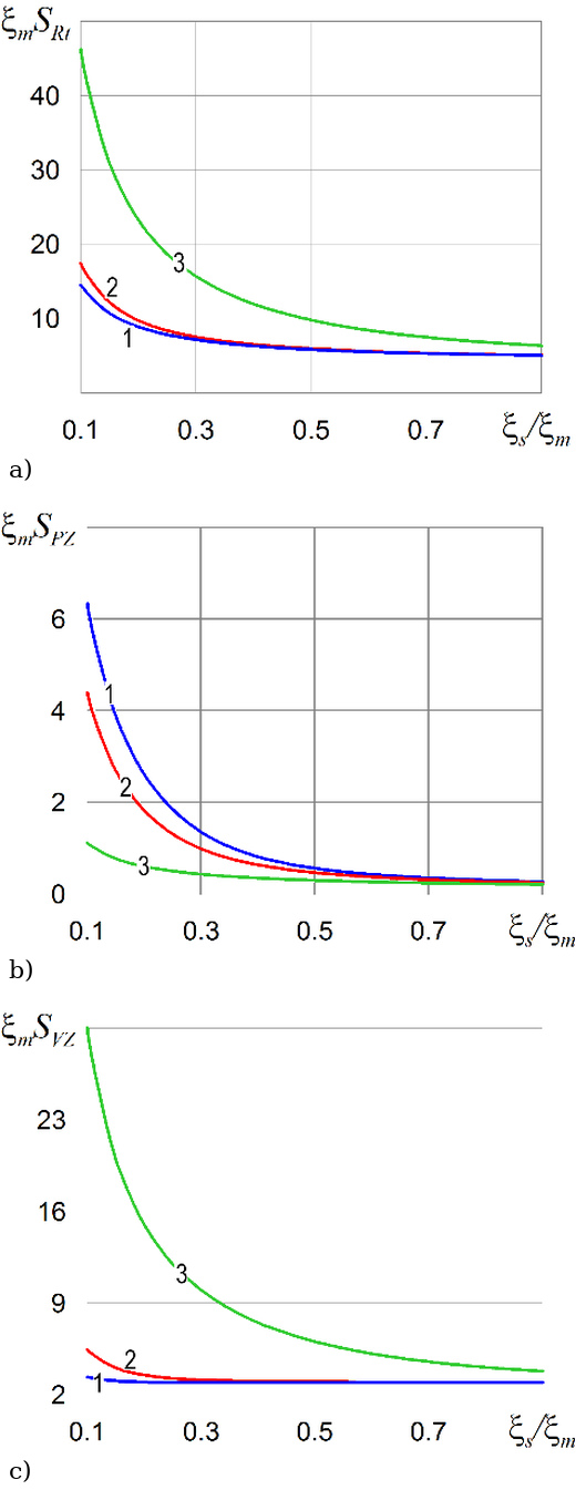
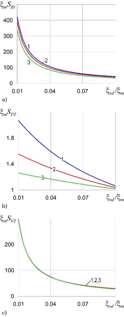
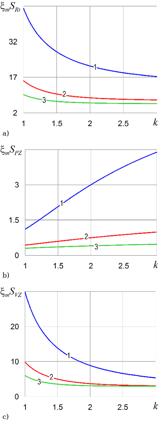
Figs. 4-6 show the effect of mass source parameters on the thicknesses of the near-surface mass density inhomogeneity zone SRt, peak zone SPZ and valley zone SVZ.

The graphs presented above demonstrate the significant potential for modeling the material curves of real surfaces using the parameters of the mass density sources. It is important to note that the parameter k enables the model to capture the peak zone, while the second term in the expression for the mass sources (10) provides effective control over the extent of the valley zone.

ELASTIC MODULI DEPENDENT ON MASS DENSITY

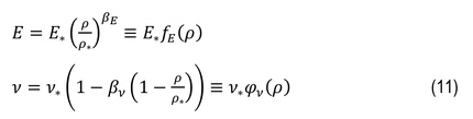
Generalizing formulas (2) for Young's modulus and Poisson's ratio, we assume

Here E*,ν* are Young's modulus and Poisson's ratio of the body material in the reference state, βE,βν are the constants. This is consistent with the literature, including [19, 25, 26].

Since mass density varies from point to point, the elastic moduli exhibit the same property. These moduli are referred to as local elastic moduli. On the other hand, Young's modulus is an experimentally measurable characteristic of a body, defined as the ratio of the applied external force intensity to the resulting relative elongation of the body (specifically, the elongation of its surface) caused by the load. The measured value represents the average over the cross-sectional area of the sample. We denote this as Eef, referring to it as the effective Young's modulus. The same considerations apply to the effective Poisson's ratio νef. A significant number of studies have been devoted to the investigation of effective moduli in heterogeneous bodies, including [27].

Using the example of a layer, we examine how the roughness of the body's real surface affects the effective elastic moduli.

THE STEADY STATE OF THE STRETCHED LAYER

Consider an isotropic solid layer, which occupies the region |x|≤l in the rectangular Cartesian coordinate system {x,y,z}. We assume that on the surfaces of the layer x=l,x=−l, which are identical, the mass density is equal to 0 and at y→±∞ the force load of constant intensity σa acts along the Oy axis.

Under such an external action, a one-dimensional situation over x variable is realized in the body

σ̂=σ̂(x),ρ=ρ(x).

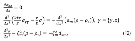
The steady state of the layer is described by the system of equations

boundary conditions

at surfaces x=l,x=−l and conditions

in arbitrary layer cross sections y = const, z = const.

We will conduct a numerical investigation for the function dsm given by the formula

Additionally, we assume (ξsl)k≫1. It can be noted that if we consider the density distribution close to the surface x=−l of a thick layer, this formula is consistent with equation (10).

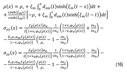
The solution of the formulated problem (11)-(15) written for the mass density and non-zero components of the stress tensor reads

where

EFFECTIVE YOUNG'S MODULUS AND POISSON'S RATIO

Based on the state equation (6) for the strain tensor we write

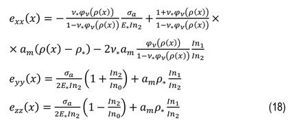
Using the solution (16), for normal components of the strain tensor we obtain

This means that the component eyy* of the strain eyy caused by external force load is

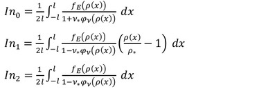
Thus, for the effective Young's modulus Eef we can write the formula

Poisson's ratio is a measure of the body size change in the transverse direction for tensile-compressive stress. Using the obtained solution and the state equation, for the component exx(σa) of strain exx caused by an external force load, we obtain

Integrating this expression over the width of the layer, we determine the average deformation exx* caused by the force load

where

According to the definition of the Poisson's ratio, using formulas (19), (22) for νef we write

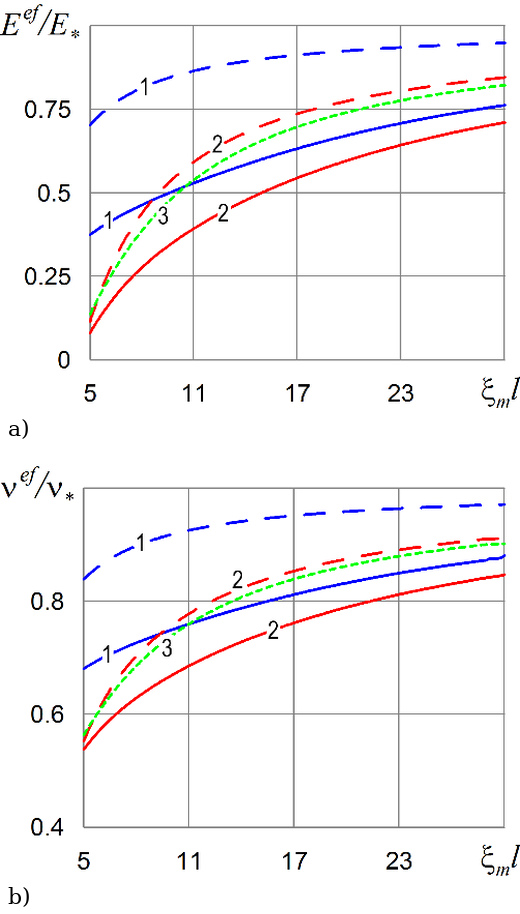
The effective elastic moduli EefE* and νefν* dependence on the layer thickness (parameter ξml) is shown respectively in Fig. 7 a) and Fig. 7 b) for ν*=0.33, k=2, ξsξm=0.8;0.2 (curves 1,2), ξsdξm=0.08, βE=1, βν=0.5, a=0.5 (solid lines), a=1 (dashed lines). The curve 3 corresponds to a=1, ξsξm=0.2, βE=1, βν=0.5, k=1. As the layer thickness increases, the value of effective elastic moduli tends toward E*,ν*. This indicates the presence of a size effect. Considering the third term in formula (15), which increases the valley zone, may lead to a significant change in the value of the effective elastic moduli. This effect is more pronounced in films with smaller thickness. Additionally, the analysis of the solution suggests that including this term increases the number of characteristic values of size effects.

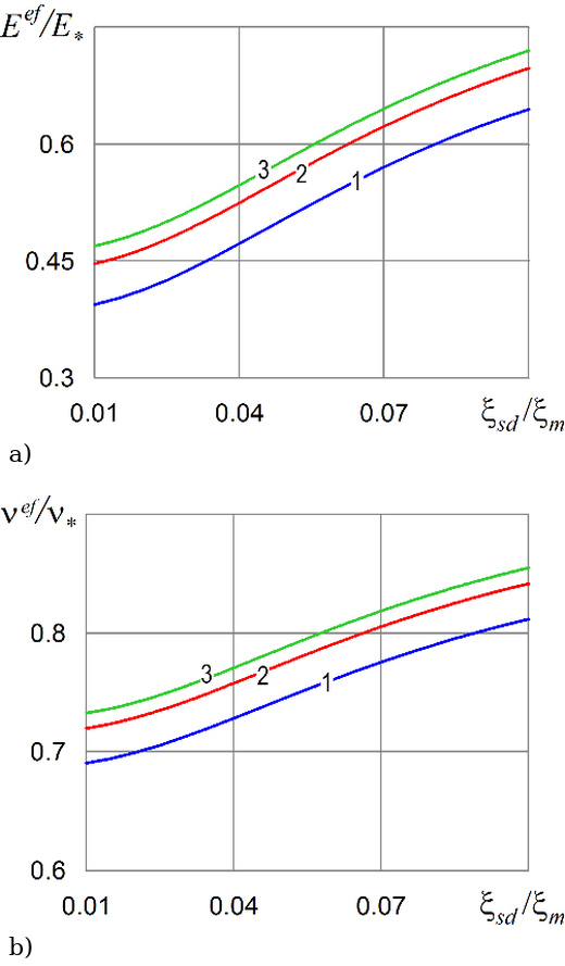
The reduction of the parameter ξsd corresponds to an increase in the valley zone as one can see from Fig. 5c. As the valley zone expands, the value of the effective elastic moduli Eef, νef decreases. This is illustrated by the graphs in Fig. 8 for the following parameters: ν*=0.33, ξml=20, k=2, ξsξm=0.2;0.4;0.8 (curves 1–3), a=0.5, βE=1, βν=0.5.

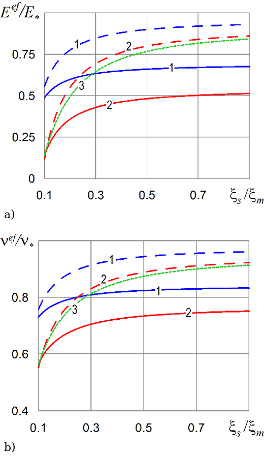
The graphs in Figure 3 c) indicate that in the region k>1, with a decrease in the value of ξs, the thickness of the peak zone increases. An increase in ξs leads to an increase in the effective elastic moduli Eef, νef for films of constant thickness. This is illustrated by the graphs in Fig. 9, which show the dependence of EefE*, νefν* on the parameter ξsξm for ν*=0.33, ξml=20,10 (red and blue lines), k=2, ξsdξm=0.08, βE=1, βν=0.5, a=0.5 (solid lines), a=1 (dashed lines). The line 3 corresponds to ξml=10, a=1, ξsξm=0.2, βE=1, βν=0.5, k=1.

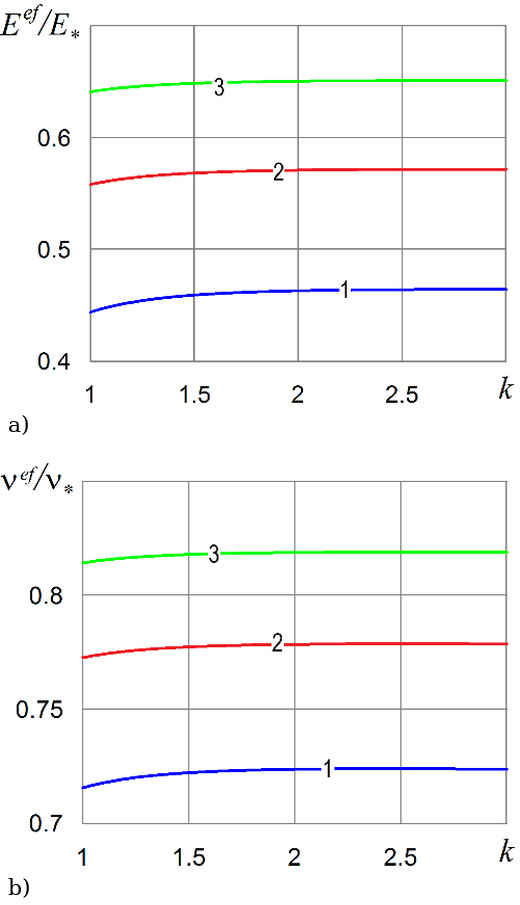
As the parameter k increases, the Young’s modulus and Poison ratio values slightly increase. This is illustrated by the graphs in Fig. 10 for ν*=0.33, ξml=10,15,20 (curves 1–3), ξsdξm=0.08, βν=0.5, βE=1, a=0.5.

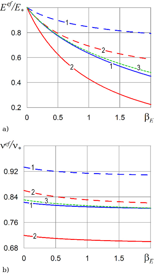
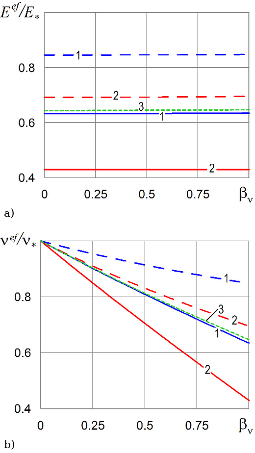
The dependence of moduli Eef, νef on the parameters βE and βν is shown respectively on Fig. 11 and Fig. 12 for ν*=0.33, ξml=20,10 (curves 1,2), k=2, ξsξm=0.3, ξsdξm=0.08, a=0.5 (solid lines), a=1 (dashed lines). The curve 3 corresponds ξml=10, k=1. On Fig. 11 βν=0.5 and on Fig. 12 βE=1. We note the practically linear dependence of νef on βν, as well as the weak dependence of Eef on βν and νef on βE.

CONCLUSION

The Abbott-Firestone curve (bearing ratio curve) is widely used in engineering practice to describe the surface texture of solid bodies. Therefore, solid mechanics models that account for surface roughness should accurately capture the characteristics of this curve. Models that incorporate the characteristics of the material curve include those developed within the locally gradient approach in thermomechanics. One of the equations in these models is the equation for mass density. In a locally inhomogeneous elastic body, the mass density equation takes the form of an inhomogeneous Helmholtz equation. When considering the roughness of the real surface of the body, the inhomogeneous term of this equation, the so-called mass sources, is selected so that the distribution of mass density reflects the distribution and regularities of the material curve. Numerical results indicate that adjusting mass source parameters allows for effective control over the mass density distribution near a nominally flat surface, as well as the sizes of the core, peak, and valley zones. Thus, by appropriately selecting mass source parameters, the profile of a real rough surface can be accurately simulated.

The effective elastic moduli, experimentally measured for thin films, reflect the properties of a real rough surface. They exhibit a size effect, meaning their value increases monotonically with film thickness, approaching the values of a medium made of identical material. The characteristic scales of these size effects depend on the material's structural heterogeneity and the sizes of the core zone, zones of peaks and valleys in the roughness profile. For thin films, the values of the effective Young's modulus Eef and Poisson's ratio νef significantly depend on the parameters of the mass sources. Any alteration in the latter, specifically, a change in the rough surface characteristics, necessitates a refinement of the effective moduli values. We note that νef exhibits a weak dependence on βE, while Eef shows a weak dependence on βν —parameters that characterize how the local Young's modulus and local Poisson's ratio vary with density, respectively.

Further research is needed to evaluate the approximations used in describing the material ratio curve, particularly the implications of neglecting the peak zone. This issue is closely related to the choice of body surface location in continuum mechanics models.