
INTRODUCTION
The induction motor (IM) is present in all industrial environments, and is the most commonly used type of motor, due to its robustness and reliability, but it is becoming increasingly complex and technical, which sometimes makes it difficult to perform optimally [1]. It is important to understand that the causes of motor and driving problems are not limited to a single field of expertise. Both mechanical and electrical problems can lead to motor failure. Therefore it is important to arm oneself with good maintenance strategies and tools to avoid costly periods of indisponibility and improve the availability of resources [2]. Bearing health is important for all machines and equipment. Several studies have shown that bearing faults account for 41% of the IM faults. When a bearing failure occurs, it has a cascading effect that significantly increases the risk of motor failure. 13% of motor failures are due to bearing failure, and over 60% of mechanical failures on a site are attributable to bearing wear [3]. Consequently, it is important to learn how to identify the signs before failure.
Accurate real-time fault diagnosis is an important means of ensuring that systems run smoothly [4]. Several failure detection techniques are used in the industrial world [5], the best known being vibration analysis which is a powerful method for diagnosing mechanical defects on rotating machines [6]. It has shown its limits when it comes to defects inducing variations in torque or defects almost imperceptible just at birth. To accurately extract the information related to these failures, the research was particularly directed towards the analysis of the stator currents of the induction motor using motor current signature analysis (MCSA) [7], [8], [9].
In intelligent machine fault diagnosis, the deep learning approach, which is an effective tool for extracting features, has attracted considerable attention from researchers [10]; however traditional artificial intelligence techniques cannot effectively discriminate complex information from raw data [11]. The shallow architectures of artificial neural networks (ANN) limit their ability to learn complex non-linear relationships hidden in measured data [12]. Involved in the data, various deep learning models have been used in fault diagnosis, such as the deep belief network (DBN) [13], [14], long short-term memory (LSTM) [15], the convolutional neural network (CNN) [16], [17] and the deep neural network (DNN) [18], [19], [20].
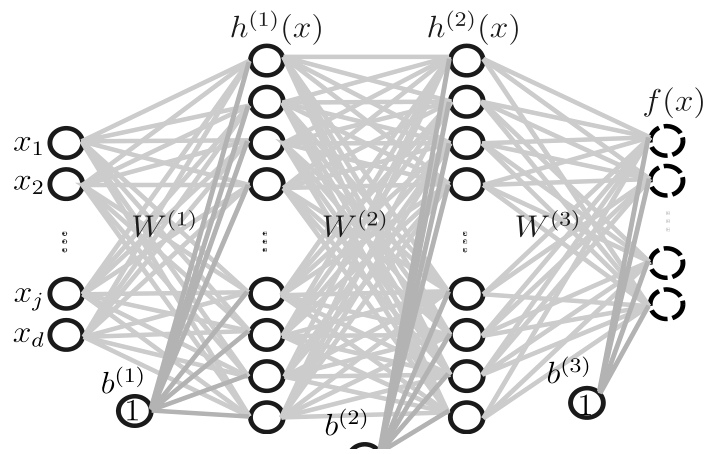
A multilayer neural network (MLP) is a common type of artificial neural network. It consists of several layers of neurons and is generally organized into three parts: an input layer, several hidden layers, and an output layer [21]. Figure 1 shows an example of a neural network with two hidden layers.
The following equations describe the operation of a neural network
with
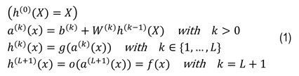
where:
The form for updating weights

with:

Where:
The most commonly used method for data normalization is the Z-score method [24]. We then used this method to transform the data such that they had a mean of zero and a unit standard deviation. This causes the data distribution to be centered around zero, with a variance of 1. The standardization formula is as follows:

where:
METHODOLOGIE
In this experimental work, we perform diagnostics on an asynchronous motor to detect possible failures. Our approach focuses on the analysis of the single-phase current of the motor to build our dataset, which will later be used to train our deep neural network (DNN) model. Fig. 2 provides an overview of the adopted methodology.
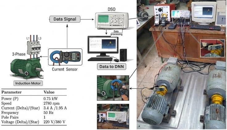
To acquire accurate and representative data on electric motor operation under a wide range of conditions, real-time measurements of the electric current in one phase of the motor were collected. Electrical signals were recorded for different operating states of the motor, including a healthy condition and several faulty conditions with deliberately induced bearing defects. The dataset consists of five classes, as illustrated in Table 1, corresponding to current signals acquired from a single phase of an induction motor. Each signal was sampled at 12 kHz and segmented into fixed-length sequences of 4000 samples. These segments represent five bearing conditions: healthy state, ball defect, inner race defect, outer race defect, and cage defect. The data were collected under various load conditions, including no load, 100 W, 200 W, and 300 W, as shown in Fig. 3, Fig. 4, Fig. 5, and Fig. 6, respectively.
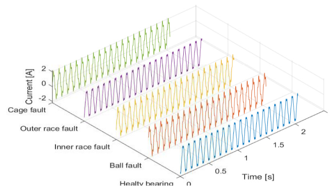
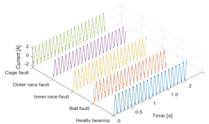
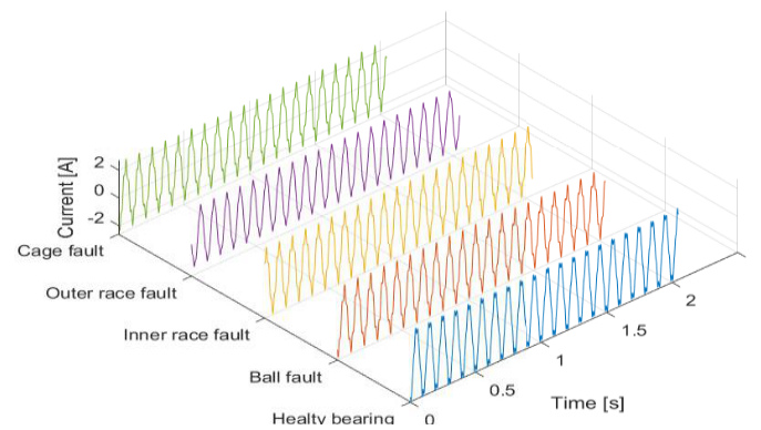
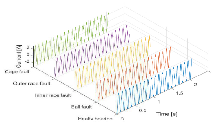
These raw data were subsequently preprocessed and subdivided into 400 segments for each class, as illustrated in Tab. 1.
Tab. 1.
Dataset Structure
The “Deep Network Designer” The Deep Network Designer application in MATLAB R2020b was used to design and implement the proposed DNN architecture. The network configuration was defined after extensive empirical tuning of its hyper parameters. Specifically, the number of neurons in the hidden layers was set to 70, the learning rate to 0.001, the number of epochs to 300, and the batch size to 256.
The selection of these hyper parameters was based on a systematic trial-and-error procedure, where multiple combinations were evaluated and compared in terms of classification accuracy and generalization performance on validation data. The final configuration was selected as it consistently achieved the best compromise between high accuracy and stable convergence, while avoiding overfitting.
The input data for the DNN model consist of ten time-domain features extracted from the segments using the Diagnostic Feature Designer application, including the mean, root mean square (RMS), shape factor, kurtosis, skewness, peak value, impulse factor, crest factor, clearance factor, and standard deviation (Std).
To improve interpretability, boxplots of three representative features of RMS, standard deviation (Std), and mean are presented in Fig. 7. These features were selected as illustrative examples from the complete set of extracted features.
As observed, the RMS and Std features exhibit a clear separation between healthy and faulty conditions, indicating their strong discriminative capability. In contrast, the mean feature shows a moderate shift between classes.
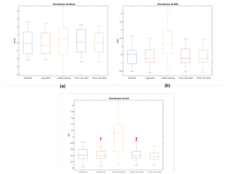
Fig. 7. Distributions of (a) mean, (b) σ, and (c) RMS standard deviation features for healthy and faulty conditions.
The data were divided into three sets: 70% for training, 15% for validation, and 15% for testing. The DNN model was designed with five outputs to identify bearing conditions. The structure of the model and chosen parameters are listed in Tab. 2.
Tab. 2.
Structure of the Deep Neural Network (DNN)
Fig. 8 illustrates all the steps described above, showing how data are divided, pre-processed and then fed into our DNN model for training.
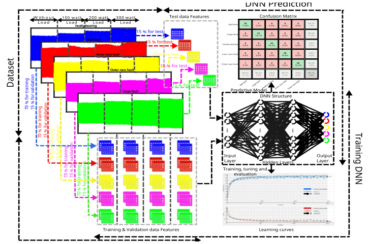
To assess the actual performance of our model, we predicted the test data and obtained an accuracy of 96.1%. Fig. 9 shows the confusion matrix, which confirms the robustness of our model for bearing failure classification. We also used our dataset to train other models such as k-nearest neighbors (KNN), vector machines (SVM), decision trees (DT), Convolutional Neural Network (CNN) and Long Short-Term Memory (LSTM) with the aim of comparing them with the DNN model.
The KNN, SVM, and DT models were evaluated using the same test dataset to assess the predictive performance of the DNN model. In contrast, for the CNN and LSTM models, each signal was partitioned into 160 segments per class.
In parallel, the one-dimensional (1D) signal segments were transformed into two-dimensional (2D) scalogram representations using the Continuous Wavelet Transform (CWT) with the Morse wavelet, following the method proposed by [16]. These representations were subsequently used as inputs to the CNN model. Finally, the raw signal segments were directly fed into the LSTM network to capture the temporal dependencies inherent in the data.
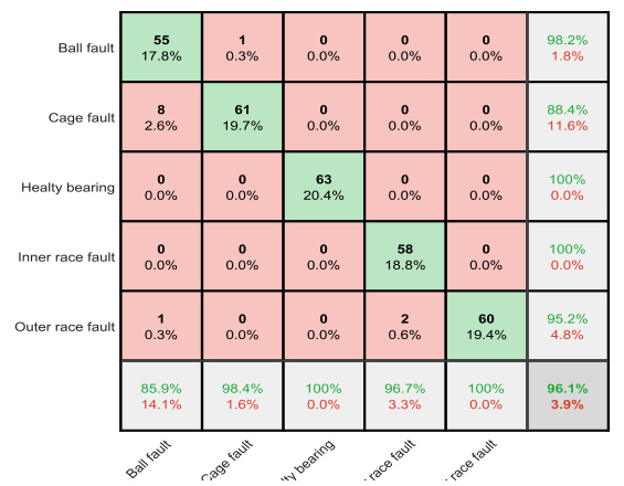
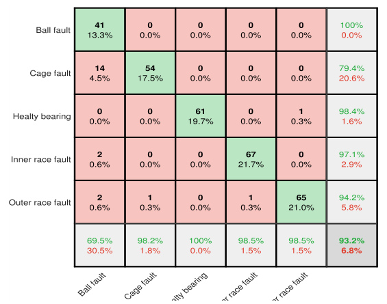
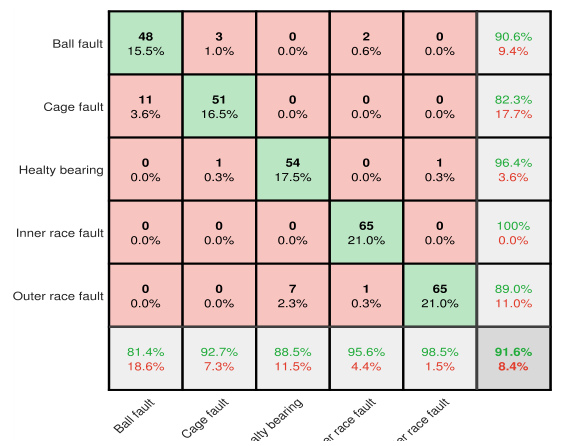
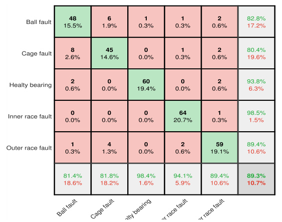
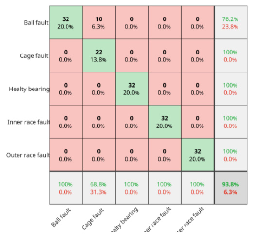
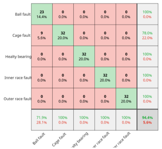
Fig. 10, 11, 12, 13, and 14 illustrate the confusion matrices corresponding to the predictions of the KNN, SVM, DT, CNN, and LSTM models, respectively. The quantitative results are summarized in Tab. 3.
Tab. 3.
In-depth comparison of the different methods
| Method | Accuracy (%) | Precision (%) | Recall (%) | F1 score (%) |
|---|---|---|---|---|
| DNN | 96,12 | 96,37 | 96,20 | 96,13 |
| KNN | 93,20 | 93,82 | 92,94 | 92,62 |
| SVM | 91,59 | 91,66 | 91,34 | 91,29 |
| DT | 89,32 | 88,94 | 89,01 | 88,95 |
| CNN | 93,75 | 95,24 | 93,75 | 93,59 |
| LSTM | 94,38 | 95,61 | 94,38 | 94,26 |
Evidence from this comparative study demonstrates that the DNN architecture is more adept at capturing complex bearing health patterns, resulting in enhanced diagnostic precision.
DNN-BASED INTELLIGENT DIAGNOSIS PROPOSED METHOD
When faults occur in the motor, a common manifestation is an increase in the phase current amplitude. However, similar variations may result from normal load changes, making the maximum current feature potentially misleading for fault identification.
To improve the robustness of the DNN model, a coefficient-based normalization is introduced to account for steady-state load levels. Coefficients C1, C2, C3, and C4 are assigned to no-load, 100 W, 200 W, and 300 W conditions, respectively, enabling the model to distinguish fault-related patterns from load-induced variations.
Assuming a monotonic relationship between load and maximum current under healthy conditions, a Min-Max normalization is applied [25] to define the coefficients as:

where: Imin and Imax – are the minimum and maximum current values under fault free conditions. This formulation constrains the coefficients within [1,k] and ensures consistent scaling across load levels.
The parameter k controls the model sensitivity: small values reduce the effect of normalization, while larger values enhance load separation but may amplify noise. A sensitivity analysis shows that moderate values of k provide the best trade-off.
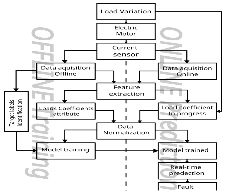
An ablation study further confirms the effectiveness of the proposed approach, demonstrating improved classification performance when the coefficients are included. Fig. 15 illustrates the overall methodology.
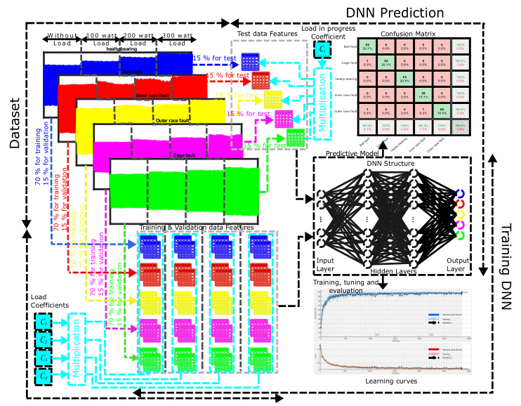
After training the DNN model offline, we developed a strategy for online prediction. When new samples are obtained, they are multiplied by the coefficient corresponding to the current load. Fig. 16 illustrates the steps of the online prediction model.
EXPERIMENTAL RESULTS AND ANALYSIS
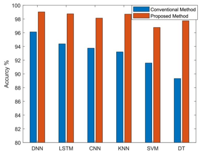
The results obtained using the proposed method are satisfactory. Fig.17 shows the results under the confusion matrix, confirming the effectiveness of the proposed method, with class identification now correct. The accuracy of the model increased from 96.1% to 99.0% using the same training and test data, ensuring a fair comparison of the performance before and after the application of the proposed method. In addition, the learning curve underwent significant improvement, demonstrating a better adaptation of the model to the pre-processed training data.
The proposed method was applied to KNN, SVM, DT, CNN, and LSTM models. The results obtained, compared with conventional methods, are significantly more satisfactory.
For the KNN method (Fig. 18), the accuracy increased from 93.2% to 98.7%. For the SVM method (Fig. 19), the accuracy improved from 91.6% to 96.8%. Similarly, for the DT method (Fig. 20), the accuracy rose from 89.3% to 97.7%.
For the CNN method (Fig. 21), the accuracy increased from 93.8% to 98.1%, while for the LSTM method (Fig. 22), it improved from 94.4% to 98.8%.
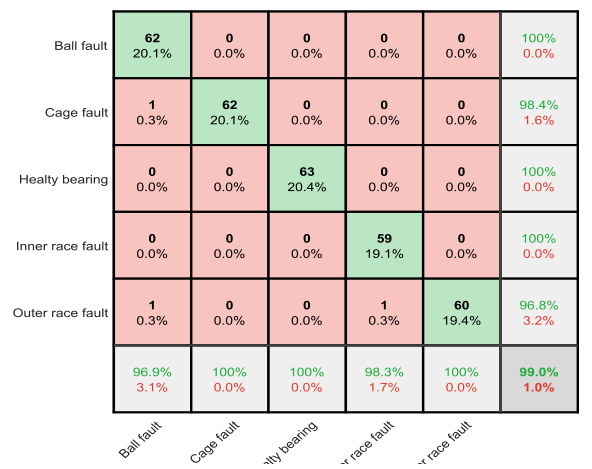
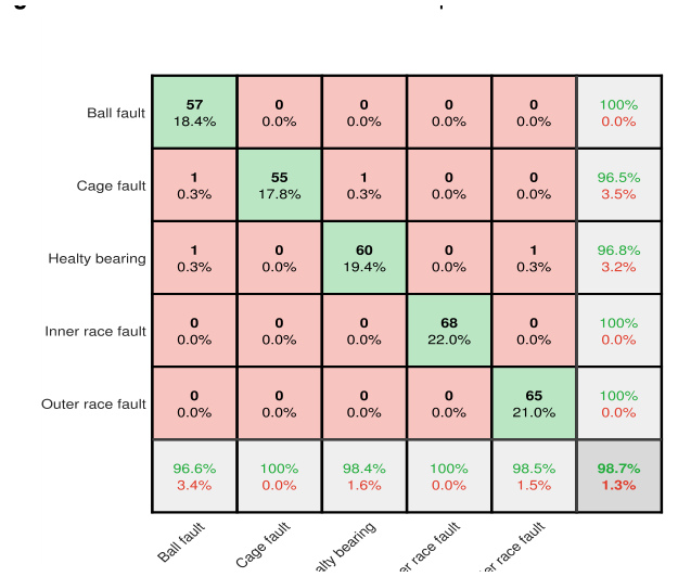
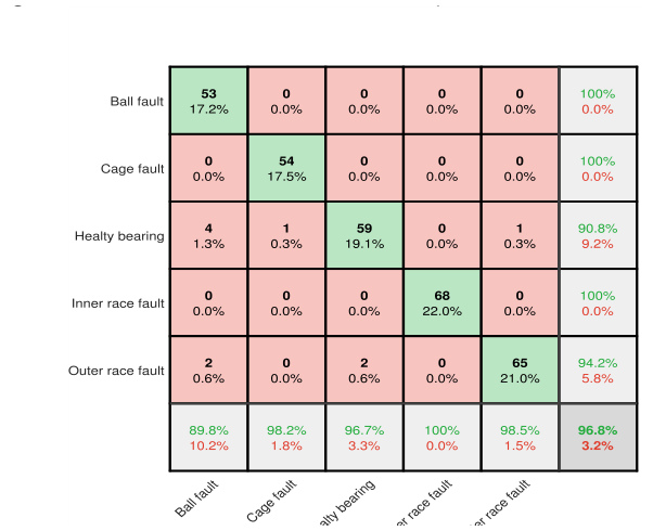
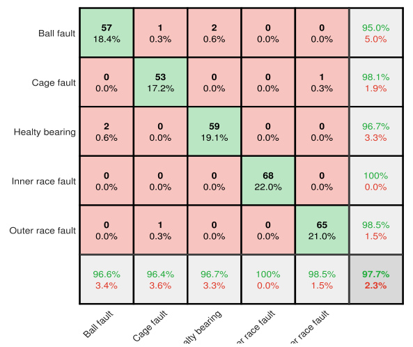
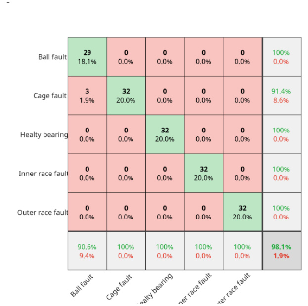
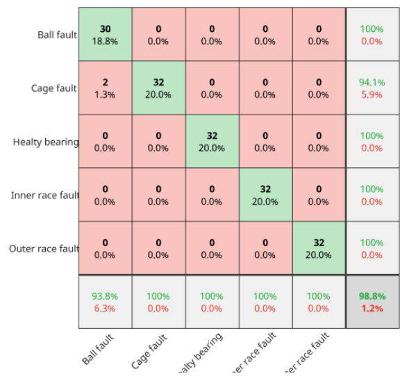
Fig. 23 shows a comparison of the different methods before and after using the proposed approach. Tab. 4 presents a more in-depth analysis and a detailed comparative performance evaluation.
Tab. 4.
In-depth comparison of the different methods
CONCLUSION
Diagnosis and predictive detection of electric motor faults are essential, and an automatic, online detection solution is the most practical way to achieve this. This is possible owing to diagnostics using artificial intelligence methods. Our work involved the application of an online intelligent diagnostic method to an asynchronous motor for the detection of bearing faults. Several techniques have been employed, including support vector machines (SVM), k-nearest neighbors (KNN), decision trees (DT), convolutional neural network (CNN) and long short-term memory (LSTM) with the aim of comparing them with the deep neural networks (DNN) model.
The approach consisted of using the current of a phase to extract the characteristics of this signal and, then using it as input for our models. The DNN model was then trained to detect and identify the bearing defects under different loads. A comparison was then made between the KNN, SVM, DT, CNN, and LSTM methods.
The proposed method demonstrates significant effectiveness in mitigating the confusion between load variations and fault signatures. To this end, a coefficient-based normalization strategy was implemented, leading to a substantial improvement in model performance. In particular, the accuracy of the best-performing DNN model increased from 96.1% to 99.0%. Substantial gains were also observed for the other models, with improvements from 93.2% to 98.7% for KNN, from 91.6% to 96.8% for SVM, from 89.3% to 97.7% for DT, from 93.8% to 98.1% for CNN, and from 94.4% to 98.8% for LSTM.
The results confirm the effectiveness of the proposed approach for fault detection by current analysis, based on a non-intrusive sensor that enables continuous monitoring without interrupting or modifying the system. The precise identification of fault classes enhances the reliability of diagnostics and predictive maintenance. Future work will focus on validation in a real-world industrial environment, with an emphasis on optimizing computational costs and simplifying integration into existing monitoring systems to ensure robustness and economic viability at scale.