
INTRODUCTION
Sliding mode control is well known for its strong robustness against different categories of disturbances and model uncertainties, and it requires only limited system information for controller synthesis compared with traditional approaches [1]. Nevertheless, its major drawback is the chattering effect, which appears as high-frequency oscillations of the system trajectory around the sliding manifold. This behavior typically arises from actuator saturation or switching delays within the controller, leading to reduced control accuracy and potentially causing early mechanical wear or elevated system temperature due to additional energy dissipation [2]. To mitigate this issue, numerous techniques have been introduced, including the boundary layer method [1], fuzzy-based sliding mode control [1], high-order sliding mode strategies [3], and the super-twisting algorithm [4 - 6].
The three-tank non-interacting process is widely deployed in industrial practice, including water treatment facilities, chemical production lines, and fuel storage operations [7], [8]. Various controllers have been proposed for liquid-level regulation in this system, such as neural-network predictive control [7], model predictive control (MPC) [8], MPC enhanced by an improved cuckoo search algorithm [9], output-feedback full-order sliding-mode regulation [10], conventional sliding-mode control [11], and optimal PI tuning using Skogestad’s approach, the Cohen–Coon method, and internal-model control [12].
Building on the super-twisting sliding mode control techniques reported in [4 - 6], this study integrates them with a fuzzy inference system to construct a hybrid control architecture. The resulting controller is implemented on the three-tank non-interacting model with the primary objective of eliminating chattering in variable-structure systems.
Recently, metaheuristic optimization algorithms have been increasingly combined with fuzzy logic systems to improve controller tuning and robustness in nonlinear and uncertain systems. Representative studies include decentralized PI-plus-fuzzy control for multivariable tank processes, interval type-2 fuzzy fractional-order fault-tolerant control, and population-based fuzzy TID control for uncertain level processes [17 - 19]. These studies demonstrate the effectiveness of optimization-assisted fuzzy control structures; however, they usually require an offline optimization stage or an additional parameter-search procedure. In contrast, the proposed F-SMC-ST controller employs a fuzzy inference mechanism to adapt the super-twisting gains online based on the tracking error and its derivative. Therefore, the proposed method preserves the finite-time convergence and robustness properties of the super-twisting algorithm while avoiding an additional offline metaheuristic optimization procedure.
The remainder of this paper is structured as follows: Section 2 details the proposed controller design; Section 3 presents simulation results and discussions; and Section 4 offers concluding remarks.
CONTROLLER DESIGN
To develop a robust and high-precision control strategy for the three-tank non-interacting process, this section presents the complete design methodology of the proposed hybrid controller. The approach integrates a super-twisting sliding-mode reaching law with a fuzzy inference mechanism to achieve fast convergence, suppress chattering, and ensure stable liquid-level tracking under disturbances and parameter variations. The controller design procedure begins with the mathematical modeling of the system, followed by the derivation of the super-twisting sliding-mode controller, and finally the construction of the fuzzy adaptation layer for tuning the super-twisting gains k1 and k2. The detailed components of this hybrid strategy are described in the following subsections.
Mathematical Model of The System
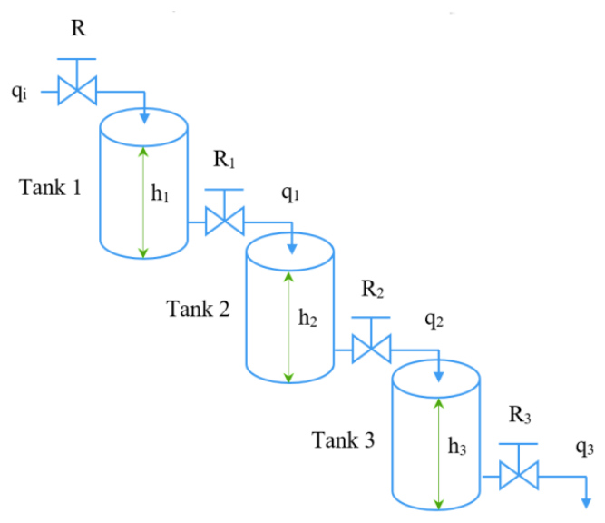
Fig. 1 shows the model of the three-tank non-interacting system [12], where the liquid flows sequentially from Tank 1 to Tank 3 through connecting pipes with resistances R1, R2, and R3. Each tank has a distinct cross-sectional area and time constant, and the level dynamics are governed by first-order flow relationships without hydraulic coupling between lateral chambers.
The mathematical model of the three-tank non-interacting system is described as follows:

where ϑ() = -1/β1x1-β3/β1x2-β2/β1x3 , ρ = R3/β1, = [x1 x2 x3]T = [h3 ḣ3 ḧ3]T is the state vector of the system, u = qi is the input signal, and h3 is the actual liquid level and (t) represents bounded external disturbances or unmodeled dynamics and |υ(t)| ≤ D, |υ̇(t)| ≤ δ.



where χ1 = A1R1, χ2 = A2R2 and χ3 = A3R3 are the time constants of tanks 1, 2, and 3, respectively.
The control objective in this study is to stabilize the liquid level in tank 3 with the proposed controller as t→∞.
Sliding Mode Control Based on The Super-Twisting Reaching Law
Sliding mode control based on the super twisting reaching law is developed to enhance the robustness and accuracy of the control system and avoid the chattering phenomenon in variable structure control [13].
Define the tracking error as (5):

where x1 = h3 is the actual liquid level and x1d = h3d is the desired liquid level of the system.
Take the 1st, 2nd, and 3rd derivatives of both sides of (5), we have (6), (7), and (8):



The sliding surface is defined as (9):

where ci(i = 1,2) must satisfy Hurwitz condition, ci(i = 1,2) > 0.
Taking the derivative of (9), we get (10):

Substitute (8) into (10), we have (11):

With the super twisting reaching law as (12) [14]:

where k1 > 0, k2 > 0.
The sliding mode control based on the super twisting reaching law (SMC-ST) for the three-tank non-interacting system is (13):

To prove the finite-time stability and exact convergence of the proposed Super-Twisting sliding mode control system in the presence of perturbations, a strict quadratic Lyapunov approach is employed.
By substituting the control law (13) into the time derivative of the sliding surface (11), the closed-loop sliding mode dynamics can be expressed as:

Let us introduce a new auxiliary variable to incorporate the perturbation: z̃ = z + υ(t). Assuming that the time derivative of the uncertainty is bounded such that |υ̇(t)| ≤ δ (where δ > 0), the error dynamics (14) is rewritten as:

Let us define the non-smooth state vector ξ = ⌈ξ1 ξ2⌉T∈ℝ2 as:

Taking the time derivative of ξ, the state-space error dynamics can be represented in a compact matrix form:

where the system matrices AB and CD are defined as:

Consider the candidate strict Lyapunov function V(ξ) in the following quadratic form:

where ef is a symmetric and positive-definite matrix (ef = efmn > 0) selected as:

The full algebraic expansion of the Lyapunov function (19) is given by:

Taking the time derivative of V(ξ) along the trajectories of the system (17) yields:
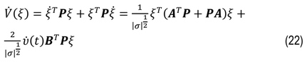
By computing the nominal matrix term, we have:

Next, the perturbation term can be upper-bounded using the condition |υ̇(t)| ≤ δ and the definition of CD and ef:

By applying the standard Young's inequality 2|ξ1||ξ2| ≤ k1ξ12 + 1/k1ξ22, the perturbation term is bounded by a quadratic form of ξ:

Substituting (23) and (25) into (22) yields the final upper bound for the Lyapunov derivative:

where the matrix gh is defined as:

To guarantee the positive definiteness of gh (gh > 0), the controller gains k1 and k2 must be strictly chosen to satisfy the following design conditions:

According to Rayleigh's quotient and the properties of quadratic forms, we have:

Since ξ12 = |σ|, it implies that |σ|1/2 ≤ ‖ξ‖.
Therefore, 1/|σ|1/2 ≥ 1/(‖ξ‖) . Using these relationships, inequality (26) can be rewritten as:
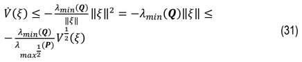
Equation (31) can be expressed in the standard finite-time differential form:

where γ = (λmin(gh))/(λmax1/2(ef)) > 0, and λmin(.), λmax(.) denote the minimum and maximum eigenvalues of the respective matrices.
Consequently, according to the Lyapunov stability theory, the sliding variable σ and its derivative σ̇ are guaranteed to converge to zero exactly within a finite time T, bounded by:

This completes the proof.
To ensure that the fuzzy adaptation mechanism always satisfies the above stability conditions, the outputs of the fuzzy inference systems are constrained by lower-bound saturation as follows: k1(e, de) in [k1min, k1max] and k2(e, de) in [k2min, k2max], where k1min = 5σ + ε1, ε1 > 0, and k2min > max{0, (σk1min − )/4} + ε2, ε2 > 0. Hence, for all admissible values of e and de, the fuzzy-generated gains k1 and k2 satisfy the sufficient stability conditions in (28). This guarantees that the Lyapunov derivative remains negative definite and that the sliding variable converges to zero in finite time. Since the sliding surface is selected as a Hurwitz polynomial, the tracking error and its derivatives are also bounded and converge to zero.
Fuzzy Logic Control
The stability requirement in (13) is fulfilled by the coefficients k1 and k2. In this work, a fuzzy inference mechanism is employed to compute these two parameters in (13), forming a hybrid structure referred to as the Fuzzy Sliding Mode Controller based on the Super-Twisting Reaching Law (F-SMC-ST). Using linguistic variables and a predefined rule base [15 - 19], the fuzzy system adaptively adjusts k1 and k2 from the feedback signals to maintain precise level regulation in the three-tank non-interacting process.
To formalize the fuzzy adaptation mechanism, the parameters k1 and k2 in (13) are expressed as nonlinear mappings of the tracking error e and its derivative ė: k1 = FIS1(e,ė), k2 = FIS2(e,ė).
Each fuzzy inference system (FIS) uses two input variables— e and —normalized within the range [−1,1], [−1,1]. Five standard triangular membership functions (NB, NS, ZE, PS, PB) [17 – 19] are assigned to each input, forming a compact yet expressive representation of system dynamics. This configuration yields 5×5=25 rules, providing a balanced trade-off between computational cost and approximation capability.
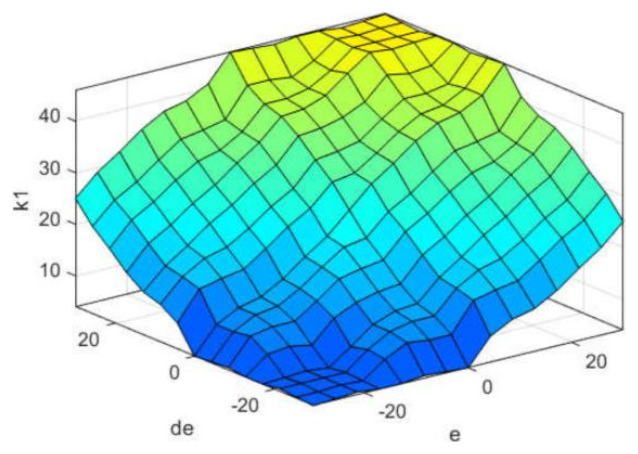
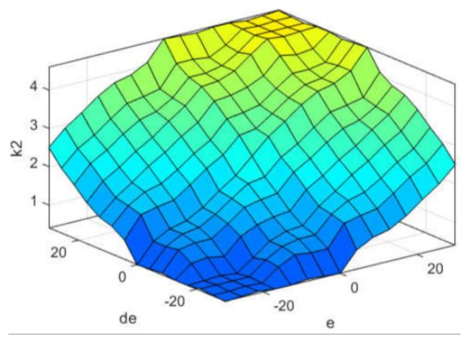
The fuzzy controller receives two inputs: the error e and its rate of change de. Both inputs are described using the linguistic sets NB (Negative Big), NS (Negative Small), ZE (Zero), PS (Positive Small), and PB (Positive Big). The complete rule base of F-SMC-ST, consisting of 25 inference rules, is provided in Tab. 1 to determine the corresponding output actions. Fig. 2(a)-(d) shows the membership functions of the input variables e and de, as well as the output functions for k1 and k2. The resulting characteristic surfaces of k1 and k2 are depicted in Fig. 3 and Fig. 4.
The selection of five linguistic terms per input is motivated by their ability to capture nonlinear variations in water-level dynamics without increasing rule-based complexity. Fewer than five terms reduce approximation accuracy, while more than five sharply increase computation and may introduce redundancy. Therefore, the symmetrical 25-rule structure provides a suitable compromise between control smoothness and real-time feasibility.
The output variables k1 and k2 use triangular or trapezoidal membership functions with monotonic ordering to ensure consistent and non-oscillatory adaptation of the super-twisting gains.
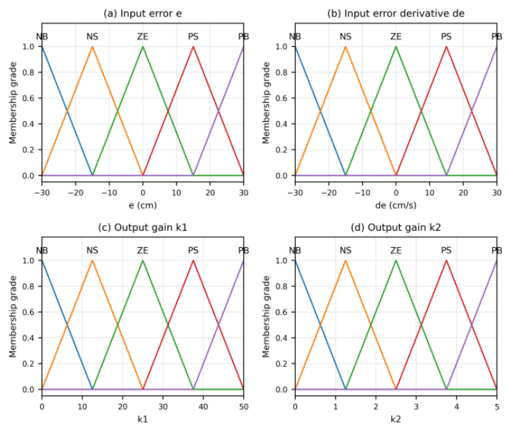
Fig. 2. Membership functions of the fuzzy inference system: (a) input error e; (b) input error derivative de; (c) output gain k1; and (d) output gain k2
The defuzzification stage employs the centroid-of-area (COA) method:

where μi(z) represents the aggregated membership function of output ki.
The centroid method is selected due to its smooth output and robustness to rule overlap, which is particularly beneficial for ensuring stable adaptation of the super-twisting control gains under disturbances and parameter uncertainties.
The fuzzy adaptation mechanism dynamically adjusts k1 and k2 based on real-time changes in e and ė. When ∣e∣ or ∣ė∣ increases, the fuzzy system increases the gains to accelerate convergence; conversely, near the sliding surface, the gains are reduced to suppress chattering. This modulation enables the controller to achieve fast transients while maintaining smooth control action, which is not possible with fixed-gain super-twisting algorithms.
Figs. 3 and 4 illustrate the resulting characteristic surfaces, showing how the gains smoothly vary across the e-de domain.
SIMULATION RESULTS AND DISCUSSIONS
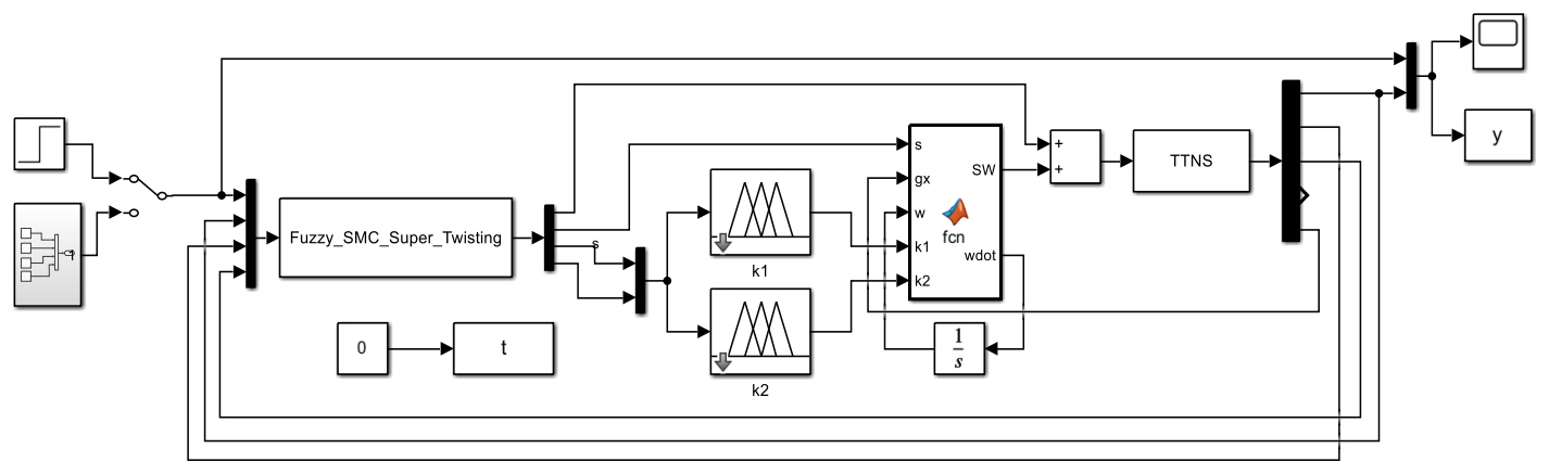
In this section, the proposed controller has been simulated and verified using MATLAB/Simulink. The simulation schematic of the proposed controller for the three-tank non-interacting system in MATLAB/Simulink is presented in Fig. 5.
The parameters of the system are used in MATLAB/Simulink as follows: A1 = 95.033(cm2), A2 = 95.033(cm2), A3 = 95.033(cm2), χ1= 44.0002(s), χ2= 61.9615(s), χ3= 80.0178(s), R1 = 0.463(s/cm2), R2 = 0.652(s/cm2), and R3 = 0.842(s/cm2).
To guarantee that the system states converge to the sliding surface in finite time, the gains must satisfy the reaching condition: σσ̇ ≤ -η|σ| (where η > 0). Tuning procedure as follows:
Step 1: if σ → 0, parameters c1 and c2 should be selected so that the polynomial s2 + c2s + c1 is Hurwitz, where s is the Laplace variable.
Step 2: To guarantee that the polynomial s2 + c2s + c1 is Hurwitz, the eigenvalues of the characteristic polynomial should have negative real parts. For κ > 0 in (s + κ )2 = 0, we obtain s2 + 2κs + κ2 = 0. Therefore, c2 = 2κ and c1 = κ2.
Based on these constraints, the specific value selected for the simulation experiment is κ =2.5. Now, we get c1 = 6.25, c2 = 5.0.
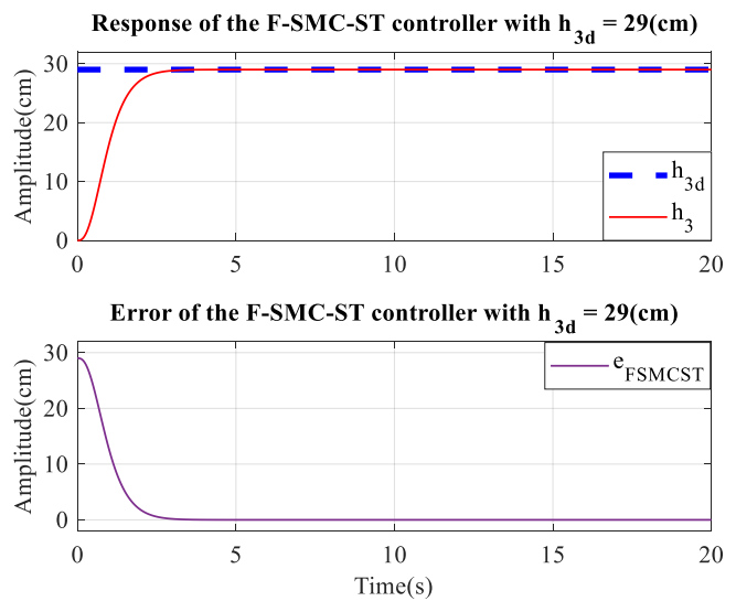
Fig. 6 illustrates the system response and tracking error obtained with the F-SMC-ST controller applied to the three-tank non-interacting model. As depicted, the liquid level in the third tank (h3) reaches the reference level (h3d = 29 cm) smoothly, exhibiting neither overshoot nor steady-state deviation. The rise time is measured as 1.6385 s, while the settling time is 3.0398 s. The computed IAE and ITAE values are 12.37 and 19.58, respectively. These performance metrics are summarized in Tab. 2 and compared with several existing approaches, including the neural network predictive controller [7], the fuzzy logic controller [20], the PID-Fuzzy scheme [20], and the PID controller tuned via the Amigo rule [20]. The AMIGO-PID rule is used as a robust and widely recognized representative for process-control benchmarking, not as an exhaustive comparison with all possible PID tuning rules. The results indicate that the proposed F-SMC-ST controller achieves faster transient response, zero overshoot, zero steady-state error, and a substantially reduced ITAE compared with the selected benchmark controllers, while its IAE remains competitive. The performance improvement is mainly attributed to the super-twisting algorithm, which suppresses chattering and improves finite-time tracking, combined with fuzzy logic that adapts the gains to system nonlinearities.
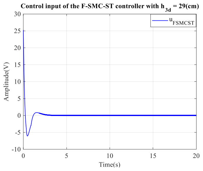
The corresponding control input generated by the F-SMC-ST method is shown in Fig. 7. This figure demonstrates the controller’s capability to effectively suppress the chattering phenomenon typically associated with classical sliding-mode control [21], achieved through the integration of the fuzzy system with the super-twisting reaching law.
Although a Mamdani-type FIS is used in this study, alternative structures such as the Takagi–Sugeno–Kang (TSK) model or adaptive neuro-fuzzy inference system (ANFIS) could further enhance adaptation accuracy. These models offer smoother gain surfaces and lower computational cost. Future work may incorporate these advanced fuzzy schemes to optimize the controller’s performance under broader operating conditions.
Tab. 2. Quality criteria of the F-SMC-ST controller
| Quality criteria | Rising time (s) | Settling time (s) | Overshoot (%) | Steady-state error (cm) | IAE | ITAE |
|---|---|---|---|---|---|---|
| Proposed controller (F-SMC-ST) | 1.6385 | 3.0398 | 0 | 0 | 12.37 | 19.58 |
| Fuzzy logic controller [20] | 25 | 37 | 0 | - | 16.8 | 181.1 |
| PID-Fuzzy logic controller [20] | 19 | 29 | 0 | - | 12.15 | 92.8 |
| PID with Amigo rule [20] | 13 | 42 | 17.1 | - | 10.34 | 96.28 |
| Neural network predictive controller [7] | 2.524 | - | 4.73 | - | - | - |
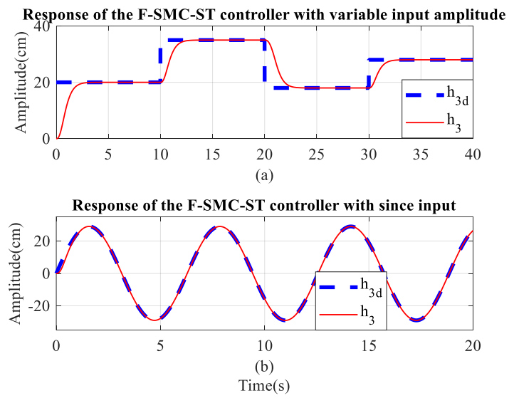
The system’s h3 response under the F-SMC-ST controller is also able to track the reference signal when h3d is shaped as either a square wave or a sinusoidal input, maintaining zero steady-state error as illustrated in Fig. 8.
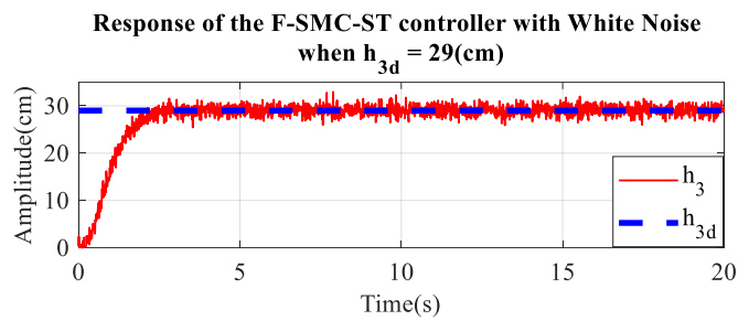
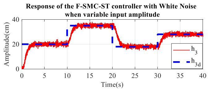
Fig. 9, Fig. 10, and Fig. 11 present the tracking performance of the proposed controller when white noise is introduced at the system output (noise power 0.01 W and sampling time 0.01 s), with the desired signals set to 29 cm, a square waveform, and a sine waveform, respectively. In all cases, the measured outputs converge to their reference trajectories within a finite time interval.
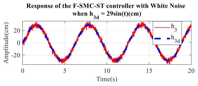
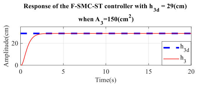
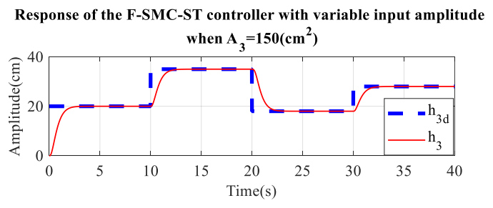
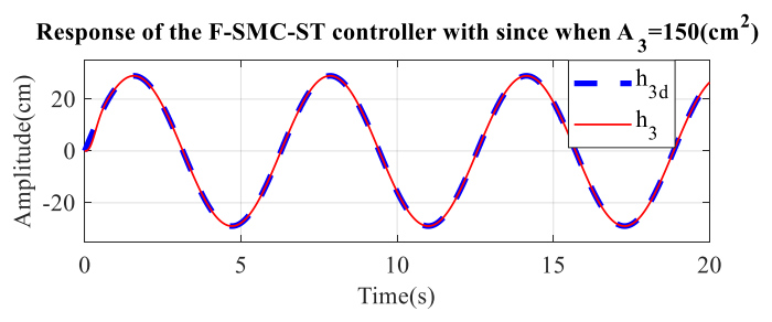
When A3 = 150 cm2 and R3 = 0.2 s/cm2, the errors between h3 and h3d converge to zero, as shown in Figs. 12-17. These results demonstrate the suitability and robustness of the F-SMC-ST controller for the three-tank non-interacting system under parameter variations.
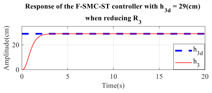
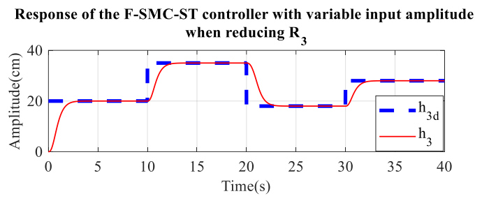
Fig. 16. Response of the F-SMC-ST controller with variable input amplitude when R₃ is reduced to 0.2 s/cm²
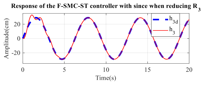
The results in Fig. 17 confirm that the proposed F-SMC-ST controller maintains accurate tracking and strong robustness under parameter variations and disturbances. Across all test scenarios, the control errors converge rapidly, demonstrating the method’s reliability for three-tank level regulation.
CONCLUSIONS
The fuzzy sliding mode control based on the super-twisting reaching law was designed in this article to stabilize the liquid level of a three-tank non-interacting system. The proposed control method enhances the robustness and accuracy of the control system and suppresses the chattering phenomenon commonly associated with traditional sliding mode control. Simulation results in MATLAB/Simulink show that the proposed controller achieves faster rise and settling times, eliminates overshoot and steady-state error, and improves the ITAE index compared with the selected benchmark controllers. Although the IAE value is comparable to those of some PID-based schemes, the overall transient and robustness performance of the proposed F-SMC-ST controller is superior under the tested scenarios. The tracking error converges to zero even when bounded output disturbances are introduced and when the parameters A3 and R3 are varied. In future work, metaheuristic optimization and advanced fuzzy structures such as TSK or ANFIS will be investigated to optimize the fuzzy system and the sliding-surface coefficients c1 and c2 under broader operating conditions.