1. INTRODUCTION

In recent days, geologists have shown their greatest interest in anisotropic media, which comes under geophysics and various branches of engineering such as earthquake and petroleum engineering and soil dynamics. Watanabe [1] discussed the deposition of typical naturally occurring soils, such as flocculated clays, varied silts, or sands, in a process called sedimentation that occurs for a long period of time. The overburden may cause the soil medium to exhibit anisotroipic and heterogeneous deformability. Sometimes, due to a different source, i.e., an explosion or other related phenomena, the energy that propagates inside or on the Earth's surface is known as elastic waves. These waves propagate in different directions from the focus point (which is also known as the epicentre), through the body or interior of the surface, known as body waves, and on the surface, called surface waves. The magnitude of the waves can be recorded with the help of an instrument called a seismograph, which is basically kept near the epicenter. The frequency of body waves is higher in comparison to surface waves.

The seismic waves are basically divided into two categories, i.e., primary waves (P-waves) and secondary waves S-waves). Primary waves move faster among the seismic waves, which are also called compressional waves since the waves are perpendicular to the surface. However, the S-waves are called shear waves, where the seismic energy transverses to medium. The body's waves are sometimes called quasi-waves due to their polarization nature, in which waves are not exactly normal or parallel to the plane (energy propagation). Gibson [2] continues the study on the above quasiwaves to calculate the impact of the depth, orthotropy, and inhomogeneity, which lie on a surface of thickness 110 ft, upon a rigid base. t the same moment, Levin [3] discovered P-wave, SV-wave, and SH-wave velocities with the help of a cross-anisotropic medium.

Gazetas [4] explored the influence of transversely isotropic half-space on the surface of the medium. In the year 2019, Vish-wakarma et al. [5] considered a fiber-reinforced viscoelastic medium and discussed the result of a shear horizontal wave under initial stress. The reference for this current work can be given to Singh et al. [6], Chaudhary et al. [7], Saha et al. [8], and Kaur et al. [9] for their advanced work towards seismic shear horizontal wave propagation. The reflection problems for the P-wave and SV-wave in a monoclinic medium at the free boundary were studied by Chattopadhyay et al. [10]. They also discussed that the incidence of the wave has a greater impact on the reflection coefficients. Wang et al. [11] and Zhang [12] have discussed the quasi SV, SH, and on P waves in a transversely isotropic medium. Reference can be given to Lu et al. ([13], [14]) for calculating traveltimes for quasi waves in transversely isotropic medium using fast sweeping method, which may be considered as an application to this current research.

Bullen [15] provided a comprehensive mathematical justification, supplemented by a heuristic proof and its subsequent validation. He further proposed an approximation for the Earth's internal density distribution, demonstrating that between depths of 413 km and 984 km, the density follows a quadratic variation with respect to depth. Beyond 984 km, extending towards the Earth's central core, Bullen approximated the density variation as a linear function of depth. He emphasized that it is reasonable to explore the behavior of wave profiles in geo-media exhibiting inhomogeneity represented as mathematical functions of depth. Numerous researchers have investigated such inhomogeneities, often modelling them as linear, quadratic, or exponential functions of the depth parameter. A limited number of studies also address quasi-wave propagation through heterogeneous substrata. In the following table, different inhomogeneity mathematical functions have been discussed. Different authors has been discussed about the quasi-wave velocities by considering various mathematical functions in terms of linear, quadratic, exponential and power law model in Young's moduli, shear modulus, and density. The following table-I has been created to give the idea of inhomogenity parameters used in varrious published works in reputed journals.

Numerous researchers have made significant contributions to addressing the issues related to body waves in cross-anisotropic soils. However, no prior work has explored the scenario where the cross-anisotropic material exhibits inhomogeneity in Young's moduli, shear modulus, and density, characterized by the following exponential function i.e. the variation has been taken in the physical quantities like Young's and shear modulus and density of the surface is e^ncosz, where n, z ∈ R of depth z. Generalized Hooke’s law of elasticity and strain-displacement relationships along with equilibrium equations of motion have been used, which further reduces to eigenvalue problem whose spectral values reflect the wave velocities. A general analytical model for the velocities of P-wave, SH-wave and SV-wave in cross-anisotropic material has been proposed. Graphical illustrations have been presented to study the influence of each inhomogeneity parameter on wave velocity against the phase angle of wave. The study may be helpful for researchers or seismologists in the field of reflection and refraction problems in body waves, which will enrich the concept of the structure of the earth's interior. Recently, a number of researchers have conducted significant studies on reflection and refraction problems in elastic media. Among them, the contributions of Sahu et al. [16], Kumar and Paswan [17], Kumar et al. [18], and Paswan and Kumar [19] are noteworthy. These studies have explored the behavior of seismic waves at material interfaces under varying geological and anisotropic conditions.

2. GEOMETRY AND SOLUTIONS

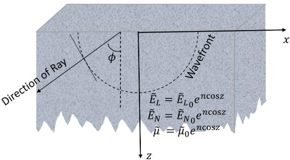
The current article studies the seismic quasi-waves in the cross-anisotropic material, with detailed calculations for the quasi-wave velocities. The problem has been discussed with the help of the coordinate system (x, y, z), where x in the horizontal direction and z in the downward direction (positive direction), shown in Fig. 1. The stress-strain relationship is as follows:

Fig. 1.

Geometry of the problem

The elastic constants may be represented as, Ẽ_L, Ẽ_N, ṽ_L, ṽ_N, and μ˜ as

Assuming the inhomogeneity in the elastic parameters as

Where, n: inhomogeneity coefficient having no dimension. From above conditions, we have

Biot’s equation of motion as follows (Biot [20])

3. DERIVATION OF PHASE VELOCITY

The following equations has been derived by substituting the stress-strain, strain-displacement relationships and the inhomogeneities in the Biot’s equation of motion.

The solutions for equations (7)-(9) can be considered as (Hu [21])

Where t=time. On putting the equations (10) - (12) in equations (7) - (9), we find

The above equations (13)-(15) can be written as follows

It gives rise to an eigenvalue problem for an in homogeneous cross-anisotropic medium and the solution of which gives the magnitude of velocities of three quasi-waves as (V_SV, V_SH, V_P) for an inhomogeneous cross-anisotropic medium

Equation (16) is the required velocities i.e SV, SH and P-waves.

4. PARTICULAR CASE

When n → 0, equation (16) reduces to

On reducing the inhomogeneity constants of eqn. (16) to zero, i.e., n → 0, this model will reduce to the model designed by Daley and Hron [21] and Levin [22]), and the results match their results, which is given in eqn. (17).

5. NUMERICAL AND GRAPHICAL REPRESENTATION

In this section, the results of the inhomogeneity parameter and the rigidity μ˜0 on the velocities of (V_SV, V_SH, V_P) waves have been discussed. On performing the numerical simulations, different graphs have been plotted for Eq. (16) and Eq. (17). The study was basically carried out to find the impact of the different parameters on varying the depth parameters z = 1 m and z = 3 m. The comparison has been shown through graphs for these (V_SV, V_SH, V_P) waves.

The current investigation deals with two sets of graphs, i.e., Fig. 2 and Fig. 3. In Fig. 2, the study has been done for all three quasiwaves, i.e., V_SV-waves, V_SH-waves, and V_P-waves. The main intention is to find the influence of the inhomogeneity parameter n (which varies as (n =-0.2, 0.0, 0.2) on the phase velocity of the (V_SV, V_SH, V_P) waves. Let us consider the first figure of Fig. 2, i.e., the V_SV-wave, in which it can be observed that the velocity decreases from 0 degrees to nearly 60-degree and then suddenly goes up and meets at the phase velocity 1.0. In the figure, it is clearly visible that the depth parameter has a significant effect on the phase velocity; the influence in the case of z = 1 m quite greater than that of z = 3 m. Again, on considering the V_SH-wave, it has been found that on increasing the phase angle, the phase velocity seems constant up to 76-degree and then suddenly jerks up and down and meets at 1.0. Here, we can also say that the influence of the inhomogeneity parameter decreases with increasing depth. Finally, the last figure in Fig. 2 has been plotted for the V_P-wave for both the depth parameters z = 1 m and z = 3 m. The study shows the increasing nature of the phase velocity for the increasing inhomogeneity parameters. The effects are visible to the naked eye, and for all three velocities, one can conclude that by increasing the inhomogeneity parameter n, the phase velocity decreases at a particular phase angle.

Fig. 2.

Dimensionless phase velocity Vs. phase angle and to find impact of the inhomogeneity parameter n on the velocity of SV, SH, and P waves

Fig. 3.

Dimensionless phase velocity Vs. phase angle and to find impact of the inhomogeneity parameter μ˜0 on the velocity of SV, SH, and P waves

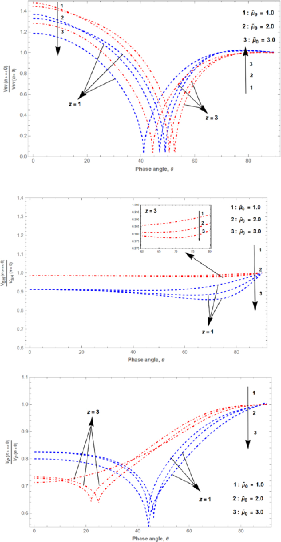
Figure 3 shows the effect of the rigidity (μ˜0) on the phase velocity of the three quasi-waves, i.e., V_SV-waves, V_SH-waves, and V_P-waves. Now taking the individual figures into the discussion, the first figure, V_SV-waves, which has been plotted for the parameter (μ˜0), gives the same effect as V_SV-wave varying for the inhomogeneity parameter n. Here, one can see that the first two curves, which have been plotted for (μ˜0=1.0,2.0), intersect at the phase angle nearly at 7 degrees. In the case of the V_SH-wave, the influence is quite significant in the case of the depth parameter z = 1 m, in which the velocity remains constant up to 40 degrees and suddenly goes up to phase velocity 1.0. And the depth parameter z = 3 m produces a very negligible effect on the phase velocity, so the zoomed figure will help to recognize the pattern of the curves. Finally, the V_P-wave, which has been plotted for the increasing values of the parameter μ˜0=1.0,2.0,3.0, creates abnormal behavior for the depth parameter z = 3 m, and for the depth parameter z = 1 m, the curve first goes down, then moves up, and finally meets at 1.0.

6. CONCLUSION

The current research work is helpful in finding a way to study the propagation behavior of body waves. The solution is carried out through a general analytical method for the three different waves, i.e., SV-wave, SH-wave, and P-wave, in a heterogeneous cross-anisotropic medium. The phase velocities of the three waves (SV, SH, and P) are obtained in closed form, as is the inhomogeneity, which is an exponential function with respect to the depth parameter z. The present study has been done for the depth of the Earth surface for z = 1 m and z = 3 m. The following are the results of this current work:

Two figures i.e., Fig. 2, and Fig. 3 have been plotted to show the impacts of the inhomogeneity parameters n and μ˜0 on the phase velocity of the SV-waves, SH-waves, and P-waves. In Fig. 2, it has been found that for all the quasi-waves, the velocity is higher near the surface, and the velocity will be negligible while moving down and down. At an angle of 90 degrees, all the curves converge to meet at the same velocity at 1.0.

In Fig. 3, which has been plotted for the parameter μ˜0, a similar type of result is found as in Fig. 2. The only difference one can note is for the SH-wave, i.e., for the depth parameter z = 3 m, the impact is quite negligible and can be observed through the zoomed figure, and for the -wave, the abnormal behavior of the curves can be detected. The findings are valuable for developing simplified calculation methods to assess the effects of seismic waves on buildings, as highlighted in the works of Ha et al. [23] and Abdoun et al. [24]. Additionally, the results can aid in quantifying wave velocities from the source, which may contribute to predicting Earth’s subsurface composition. Furthermore, this approach can assist in identifying oil traps and other economically significant geological formations. The study may be helpful to geologists to know the presence of different materials present inside the earth surface.