
Introduction
Walking stability remains a significant challenge in biomechanical engineering, particularly for populations with mobility impairments [1]. Recent advancements in computational musculoskeletal modeling have highlighted the role of joint mechanics in developing assistive technologies [2]. Consequently, understanding natural joint kinematics has become crucial for engineering applications in rehabilitation and assistive device design [3-5].
The knee joint, as the largest and most complex synovial joint in the human body, presents substantial engineering challenges due to its intricate geometry and dynamic loading conditions [6]. Computational modeling offers promising solutions through prosthetic design and exoskeleton development. For exoskeletons in particular, safe human-robot interaction requires accurate biomechanical models [7-8].
This paper presents a multibody dynamics approach for knee joint modeling that incorporates musculoskeletal elements. The proposed framework simulates knee joint kinematics and contact forces during dynamic activities. The human body can be modeled as a biomechanical system primarily through two methodologies: the Finite Element Method (FEM) and Multibody System (MBS) simulations. The latter is commonly implemented for analyzing gross motions and complex environmental interactions [9-10]. In contrast, FEM is typically employed under quasi-static loading conditions to predict stresses through accurate geometrical modeling of contact surfaces [11]. Since human gait is a gross-motion activity, it is predominantly analyzed using MBS formulations, which are also favored for dynamic loading conditions due to their computational efficiency and simplicity [12-13].
Over recent decades, numerous theoretical and experimental studies have been dedicated to knee joint simulation [14-30]. Research in this field can be divided into kinematic and dynamic approaches. Kinematic models describe the motion between the femur and tibia without considering applied forces and torques, whereas dynamic models predict the forces between articular surfaces, ligaments, and muscles.
The multi-body dynamic knee model was first proposed as a four-bar linkage comprising a rigid femur-tibia complex, two ligaments, and a meniscus [18]. Subsequent improvements incorporated curves representing the articular surfaces of the femur and tibia [19]. To model soft tissues, the viscoelastic nature of knee contact was investigated using Kelvin and Voigt contact-force models [20]. For enhanced modeling accuracy, FEM and quasi-static approaches were utilized to analyze knee behavior [21-22].
Further developments included dynamic models that treated the knee as two rigid bodies (tibia and femur) connected by nonlinear springs representing ligaments [23]. Three-dimensional analysis advanced with studies considering the femur and tibia as contacting bodies with ligament constraints, using spherical and planar surface approximations [24]. As research progressed, comprehensive three-dimensional models incorporating soft tissues and experimental validation emerged [25], followed by meniscus modeling in ADAMS software [26]. Additionally, collision detection and surface distance determination tools were developed for dynamic simulation [27].
In contrast to studies using static loading for knee contact force analysis [29], recent research has combined musculoskeletal models with extended knee models for gait cycle simulation. This integration aims to improve biomechanical joint modeling through enhanced geometric representation and contact models for soft tissues. For instance, some studies have combined musculoskeletal models with MBS of the knee joint [30-31], while others have integrated musculoskeletal modeling with FEM to achieve accurate solutions for knee joint dynamic behavior [32-33].
Despite the abundance of studies on three-dimensional knee models, two-dimensional modeling approaches remain preferable due to their lower computational cost [7-10, 13, 34]. Although the aforementioned 3D models offer high accuracy, they are often too computationally intensive to provide rapid feedback for gait analysis involving gross motions [9]. Furthermore, many existing sagittal plane models do not adequately incorporate dynamic loading, such as the forces generated by the musculoskeletal system during the gait cycle [9, 14, 23]. An accurate estimation of joint forces using a musculoskeletal model could significantly benefit the joint unloading treatment process.
This study introduces a novel two-dimensional knee model that features an unfixed axis of rotation, a detailed geometric representation of contact surfaces, and incorporated soft tissue properties. Tibiofemoral contact was modeled as elastic using a two-layer contact model representing cartilage and bone. In this formulation, the tibia moves relative to a fixed femur, with their relative motion governed by contact forces and interacting surfaces.
Contact mechanics were simulated using a Kelvin-Voigt viscoelastic model, while the geometric profiles of the contact surfaces were derived from knee MRI data and represented by spline functions. The model was evaluated using motion capture data from both healthy and osteoarthritic participants to analyze joint reaction forces in the sagittal plane during planar motion.
Experimental motion data served as input for OpenSim, where the standard processing pipeline—including model scaling, inverse kinematics, and inverse dynamics—was executed. This workflow enabled the estimation of knee joint reaction forces using the implemented modeling framework. The model incorporates detailed tibiofemoral joint geometry and examines its viscoelastic contact properties. Consequently, this multibody framework can simulate knee kinematics and estimate contact forces under various musculoskeletal conditions.
Section 2 presents the materials and methods, including the proposed kinematic contact model for the constrained knee joint. Section 3 details the simulation results of the novel knee model for both healthy and osteoarthritic (OA) conditions in a multibody dynamics framework, utilizing a two-layer contact approach. This section analyzes the dynamic behavior of the knee—including tibiofemoral contact force, indentation, and contact point trajectory—throughout the gait cycle.
Materials And Methods
The multibody system dynamics approach is a highly efficient method for contact mechanics analysis. Such an analysis is fundamentally divided into two categories: first, generalized contact kinematics, which includes collision detection and indentation calculation, and second, contact force models [35]. Both of these aspects are described in the subsequent sections, and the MBS methodology is explored through case studies. This section provides a comprehensive description of the methodology adopted in this study. To accurately investigate the knee joint's biomechanical behavior, a comprehensive mathematical model was developed, integrating six major components: the geometric representation of the articular contact surfaces, the formulation for contact detection, the development of a constrained knee joint model, contact force modeling, the musculoskeletal representation of the lower limb, and the direct dynamic analysis of knee motion. Each of these components is described in detail in the following subsections to ensure the transparency of the modeling approach.
Geometric Modeling of Tibiofemoral Contact Surfaces
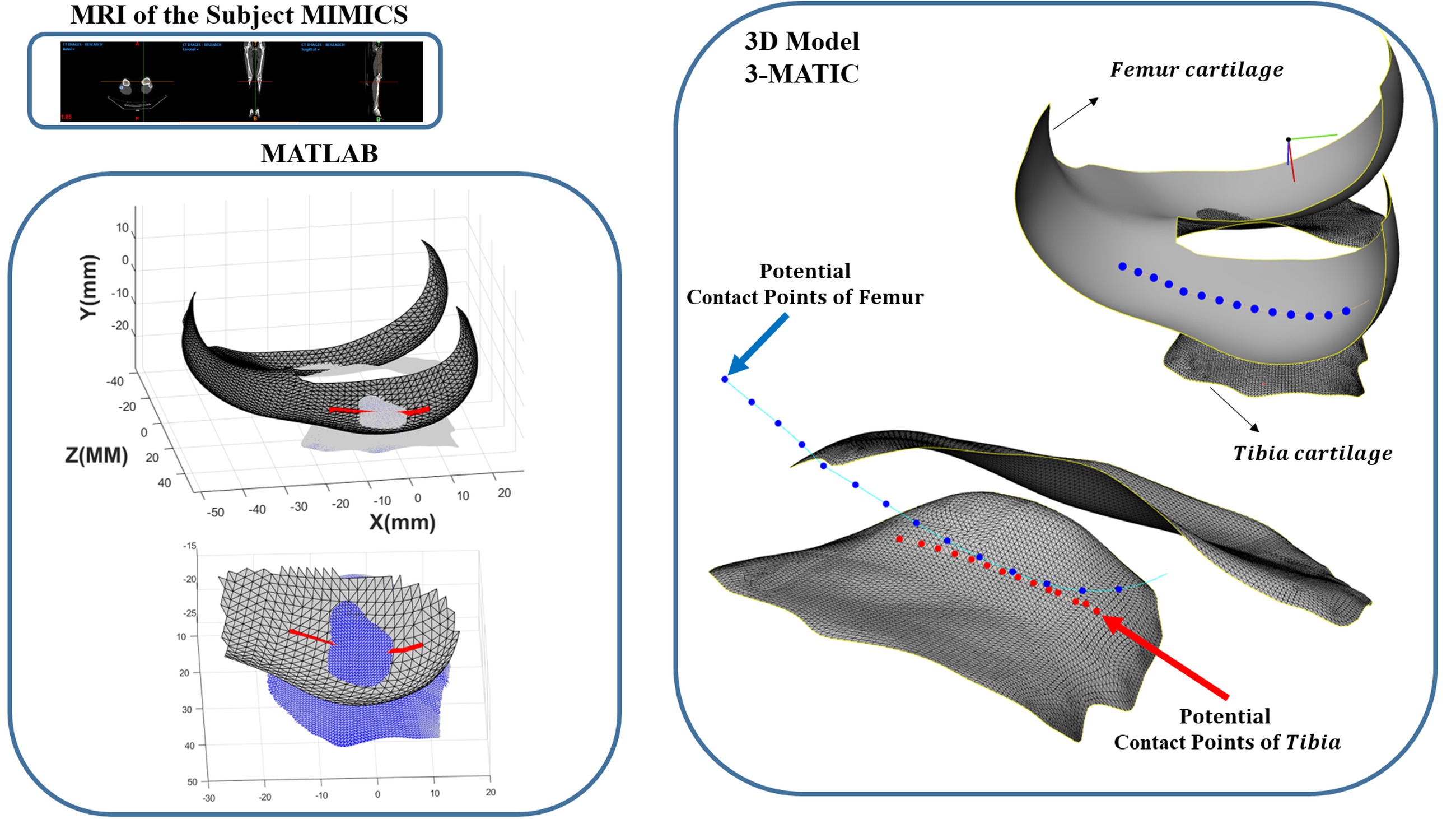
With the development of a dynamic knee model that enables analysis of tibiofemoral contact mechanics, an accurate and precise definition of the articular contact surfaces between the tibia and femur is essential and unavoidable. Therefore, magnetic resonance imaging (MRI) data of the knee were utilized to obtain detailed geometric characteristics of the joint surfaces. Based on the MRI images, two sets of data points were extracted to represent the geometry of the tibial and femoral cartilage surfaces.
To mathematically describe the overall geometry of these surfaces, curve fitting based on interpolation techniques was employed. Although several interpolation methods such as Lagrange and Hermite interpolation are commonly used [36], they are not suitable for this application due to their discontinuities, computational complexity, and incompatibility when new data points are added.
Accordingly, in the present study, a cubic spline interpolation function was adopted because of its smoothness and continuity between the connection points of partial curves. The cubic spline interpolation relies on three main conditions: (1) each segment of the curve is a third-degree polynomial with different coefficients in each interval (xi,xi+1), (2) the curve passes exactly through all given data points; and (3) the first and second derivatives are continuous at each node xi. Fig. 1 illustrates the extracted 3D model of the tibiofemoral cartilage surfaces obtained from DICOM MRI data. Following 3D reconstruction in Mimics, the coordinates of the surface contact points were precisely extracted using Geomagic/3-matic software. The MRI data were acquired using a 3.0 T clinical MRI scanner as reported in [37]. The contact regions were identified with reference to the contact point distributions reported in CT-based studies [38]. The surface equation fitting and subsequent numerical analyses were then carried out in MATLAB.
Generalized contact kinematics
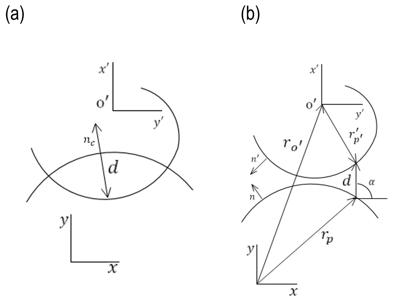
In this section, the generalized kinematics of contact between two rigid planar bodies subjected to an oblique eccentric contact is investigated. The kinematic analysis aims to define a new algorithm for collision detection. As can be seen in Fig. 2, two convex bodies with the absolute velocity of r,r' and the potential contact points of p, p' are shown. The kinematic calculation consists of three fundamental quantities known as the location of potential contact points, their Euclidean distance, and relative contact velocities [39-40]. Generally, this information should be extracted during the impact-contact phenomenon to determine the contact force. The motion of the bodies is constrained by the use of relative distance and velocity of the potential contact points. The positive and negative values of these indices represent the corresponding separation and contact modes. The two mentioned scenarios are illustrated in Fig. 2. The positive value of the relative normal velocity (penetration velocity) is the indicator of bodies in the indentation or pressure phase.
Drawing captions should be typed in Arial Narrow 9 pts., single spacing: before 3 pts., after 18 pts [4]. When using one description to several drawings, the drawings shall be denoted in the sequence: a), b), etc. Letters a), b) should be within the figure), with the description as shown in Fig. 5.
A vector that connects two points of potential contact p′, p is expressed as a distance function:

For the vector rₚ and rₚ′ in the global coordinate system considering the inertial reference frame,

where Aₖ is the rotation matrix and the r′ₚ′ is a vector in the local coordinate system. The normal vector of the contact plane (n) is shown in Fig. 2.
The magnitude of the vector d is indentation and calculated as follows:

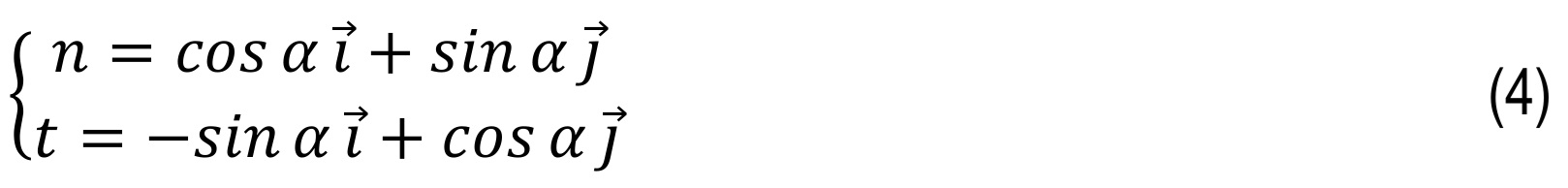
and normal and tangential unit vectors based on the contact plane are:
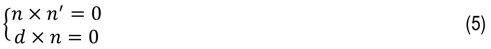
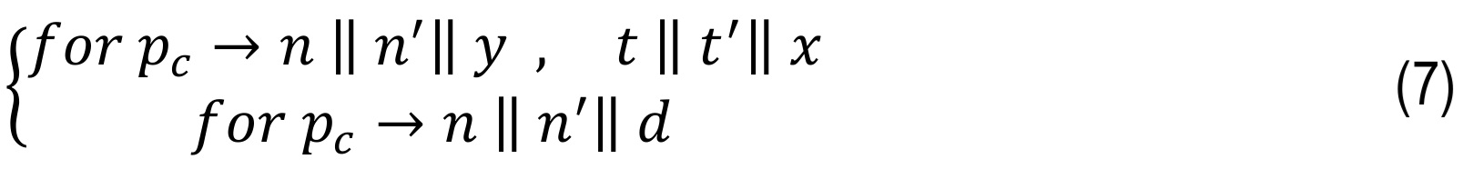
Therefore, for the representation of the maximum penetration depth by contact equation, three geometrical conditions can be defined as follows: (i) the distance between the potential contact points defined by the vector d should be equal to the minimum distance; (ii) the vector n is collinear with vector d; (iii) the n and n′ vectors at the contact potential points must be collinear. The terms (ii) and (iii) can be expressed in terms of cross-products.
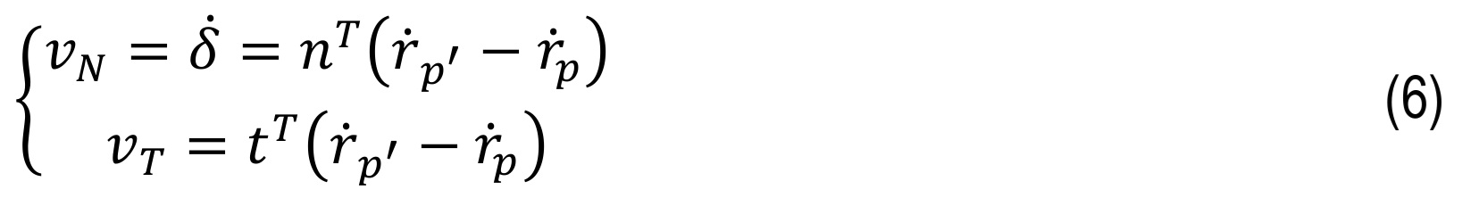
The following condition should be satisfied for the contact occurrence dᵀ n ≤ 0. For the normal and tangential velocity of the indentation:
Although this procedure seems computationally effective, it is limited to convex or flat curves with smooth surfaces. It should be noted that this approach is extendable for most geometrical modes with the unique representation of the contact tangent plane [9].
Novel constrained knee joint model
Accurate estimation of skeletal kinematics from skin markers requires defined kinematic constraints to be produced natural motion. There are several kinematic constraints used to describe the knee joint kinematics [41-42]. The three associated mechanisms and proposed knee model will be provided in this section. (1) In the ball and socket model, the knee is modeled as a spherical joint with 3 DOFs [43-44]. (2) By the hinge model, the knee is modeled as a revolute or pin joint with 1 DOF around flexion/extension axis [45]. (3) The parallel mechanism model describes the articulation through two sphere-on-plane contacts, guided by three isometric ligaments acting as connecting links [46].
The articular surfaces of the femoral condyles are convex anteroposteriorly, and the tibial surfaces are comparatively flat [10].Therefore, the proposed model is similar to the sphere-on-plane model, and it can be named curve fitted-on-plane. The novel model uses point clouds of knee MRI to produce a fitting curve of the femur. The sphere-on-plane and enhanced model are shown in Fig. 3.
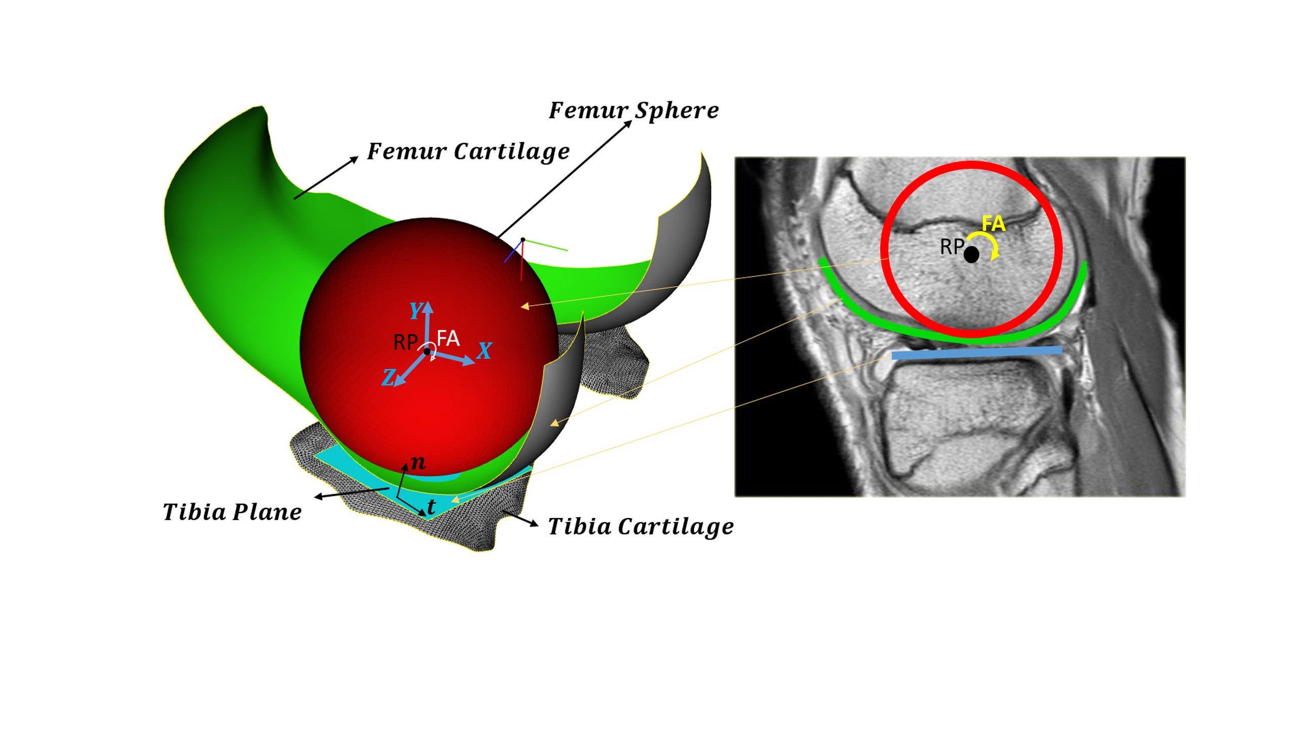
Fig. 3. The two-dimensional knee model was developed using an MRI image [10] (sagittal plane view). The biological knee model features spherical geometry, with the femoral condyles represented by developed curved surfaces defined based on the knee flexion angle (FA) and a reference point (RP)
As depicted in Fig. 3, the curve fitted on the plane model requires an algorithm that detects the collision with efficient accuracy and computational time. According to the tibia model as a plane in previous studies, in this section, the tibia surface is approximated as a plane, and the femoral surface point clouds are fitted by the spline method to provide an accurate model with less computational time. Therefore, the set of points p = [xₚ, yₚ, zₚ]ᵀ on the femur is acquired. According to the enhanced knee model, substituting n = ∞ into Eq. (5), p_c as the point of maximum penetration depth in collision geometrical condition can be recast asp, yp, zpTon the femur is acquired. According to the enhanced knee model, substituting n=∞ into Eq. (5), pcas the point of maximum penetration depth in collision geometrical condition can be recast as
It should be noted that this approach is extendable for most geometrical modes with the representation of the contact of the fitted curve-plane. The main parameter in calculating the amount of contact force is the vector d from Eq. (1) in Fig. 1 that indicates the maximum penetration depth in the tibia.
The contact force models
Collision is a common phenomenon occurring in many mechanical systems. The best-known force law for the contact force created between two isotropic materials based on the elasticity theory was introduced by Hertz [47]. This theory is restricted to surfaces with less friction and perfectly elastic solids. In this method, the contact force is a nonlinear function of indentation.
Kelvin–Voigt model includes the viscoelastic behavior and presents the behavior of a media with a series of discrete springs parallel with dampers. In other words, Kelvin– Voigt enters the effects of viscoelasticity into the elastic Hertz model. The relation between the restoring force and displacement is found using the following relation [48]:

where K is the general stiffness and C is the damping of viscous elements.

where Fₙ, Fₜ are normal contact force and friction force and eliminating friction force, normal contact force is obtained as follows:pn,Fpt are normal contact force and friction force and eliminating friction force, normal contact force is obtained as follows:

Also, the concept of pure elastic two-layer collision modeling [49] has been used for modeling osteoarthritis. Therefore, in the two-layer collision force scenario, the sum of the collision forces in each layer is obtained as follows:
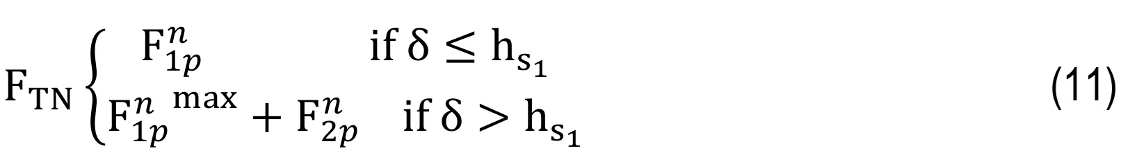
where Fₙ, Fₜ are normal contact force and friction force and eliminating friction force, normal contact force is obtained as follows:TNis the total normal contact force and F1pn,F1pnmax are the contact forces due to the penetration depth of the first layer and F2pn is the contact force due to the penetration depth of the second layer [9]. Considering viscosity, the proposed model based on the concept of viscoelastic two-layer collision modeling can be recast as follows:
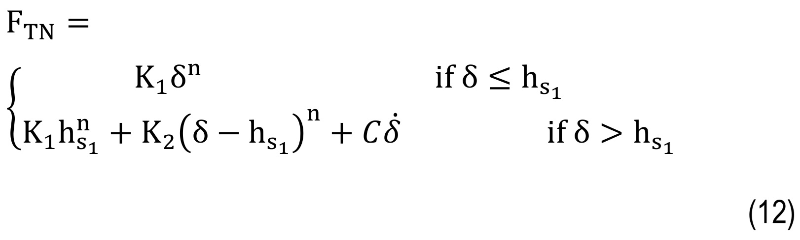
where K1 and K2 are the general stiffness of the first and second layers and hs1is the critical penetration depth.
Musculoskeletal Model
Understanding the effect of contact model parameters on knee performance, and extracting a realistic outcome of natural and healthy knee function, requires the definition of appropriate loading and kinematic constraints. Therefore, the musculoskeletal model adopted in OpenSim is used to model the motion and predict the tibiofemoral contact forces (FTN) in the knee for a full gait cycle [50].
The model uses the gait 2354 [51] model as a musculoskeletal model with 22 degrees of freedom, 54 muscle-tendon actuators, and 17 torque actuators for simulation [51]. Initially, the generic musculoskeletal model was scaled to match the anthropometry of the case study. Subsequently, joint angles were calculated using the Inverse Kinematics (IK) tool. Following this, the Residual Reduction Algorithm (RRA) tool was used to minimize the residual forces arising from minor discrepancies between the force plate data, marker data, and the musculoskeletal model. Muscle simulation was performed using the Computed Muscle Control (CMC) tool. It is noteworthy that the outputs from both IK and RRA can be used as inputs for CMC; however, in this case, the output from RRA was used as the effective input for CMC due to its solution. Finally, based on the analyses performed by the aforementioned tools, the joint reaction forces were extracted using the Analyze tool.
Forward dynamic modeling
The constitutive motion equations of tibiofemoral joints can be written based on the femur mass M, translational acceleration Z in the Newton’s second law of motion:

in which the external force Fexternal, and total normal contact force (FTN) are the vector sum of all force vectors applied to the femur as shown in Fig. 4. Accordingly, the external force (including muscle forces) defined in the model (Eq. 13) is extracted from the OpenSim analysis and applied to the reference point of the knee multi-body model.
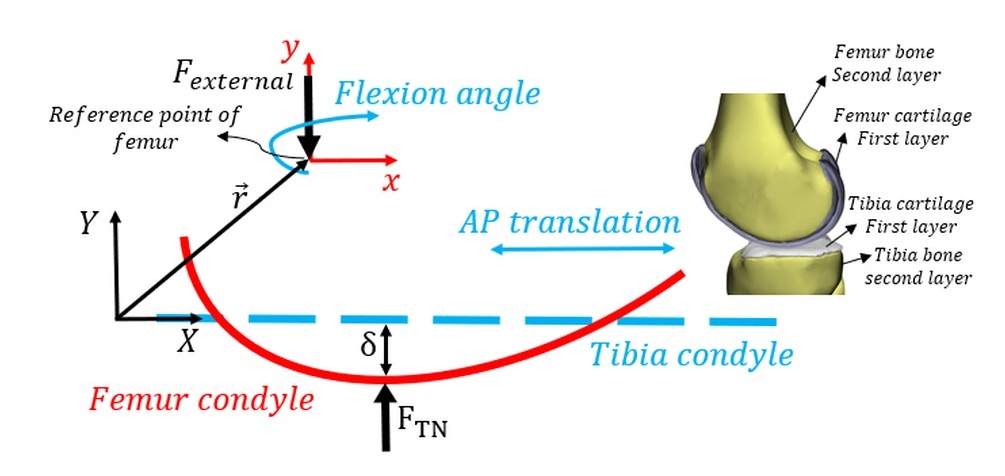
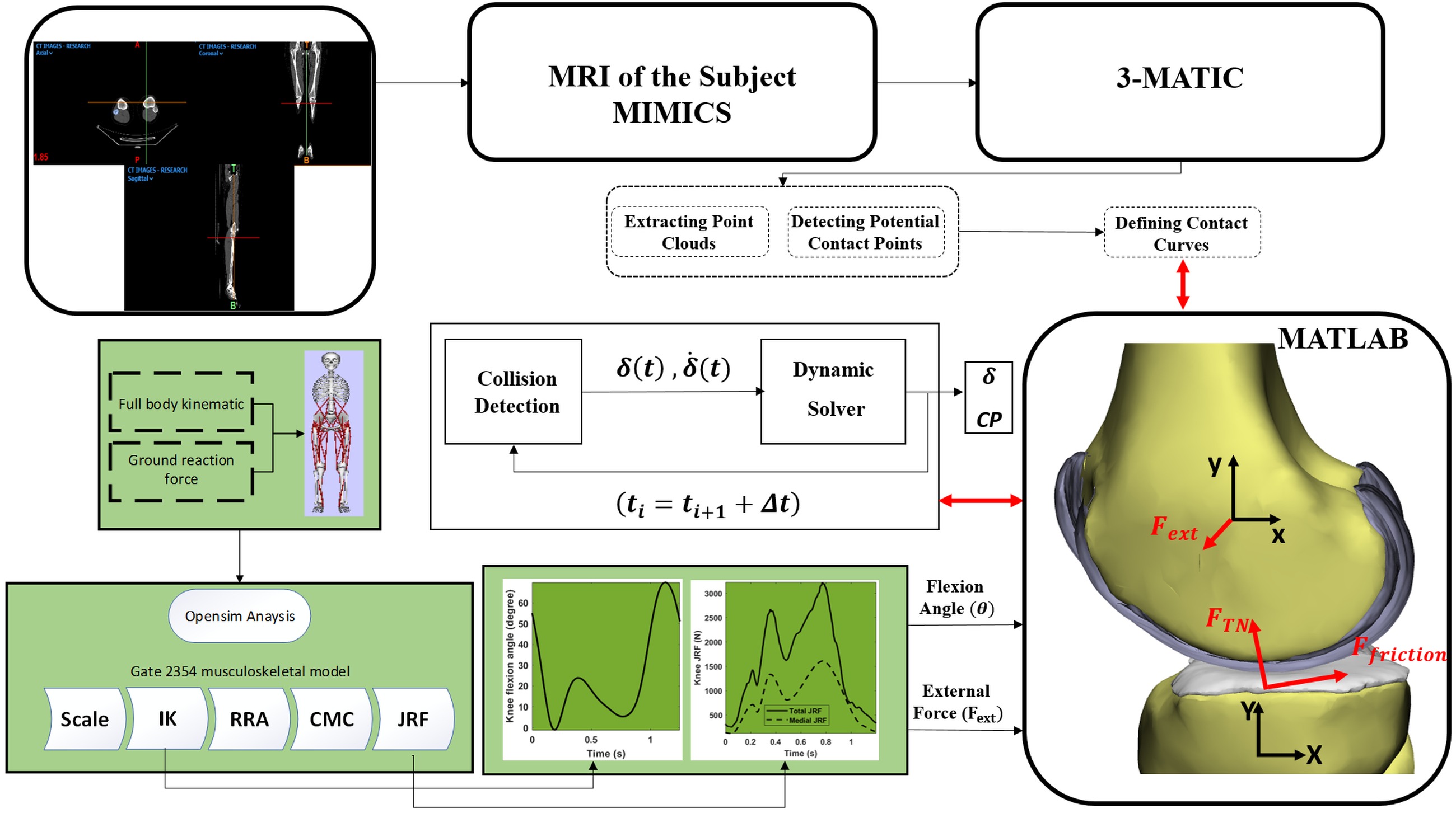
A forward dynamics model of the femur was developed, allowing free translation and rotation with 3 degrees of freedom (DOF). Within this dynamic system, two degrees of freedom—specifically the flexion-extension angle and anterior-posterior translation—were constrained using known kinematic data. The motion is defined in the sagittal plane using the (X, Y) coordinate system illustrated in Fig. 4. The values for the two constrained parameters were derived from motion capture analysis and dynamic knee MRI data [30]. The proposed methodology was implemented in a computational algorithm, with the workflow schematically presented in Fig. 5. This study focuses on quantifying tibiofemoral indentation depth during the gait cycle using a planar knee model. The model incorporates a generalized collision detection algorithm and contact mechanics formulation. The tibia was assumed fixed, while the femur was permitted translational and rotational motion within the plane. Initial conditions were obtained from the static solution of forces applied to the tibia. The outputs of the computational framework (Fig. 5) include contact force, contact points, indentation depth, and displacement of the femur’s center of mass along the Y-axis.
Results And Discussion
In this section, numerical simulation of a 2D sphere-plane model and fitted curve-plane model for human knee joint is performed. Fig. 4 presents a 2-D model of a knee with a mobile femur and fixed tibia, with the modeling performed in the sagittal plane. Due to analyzing the knee joint's behavior in the gait cycle, the dynamic multibody model of the knee has been analyzed by combining the musculoskeletal model. By understanding how a normal, healthy knee works, it will be easier to understand the performance of assistive device. The results are obtained for knee osteoarthritis (75% KOA [9]) and compared to those for the normal knee. The Kelvin–Voigt contact model is used to calculate the contact force. Table 1 presents the properties of the contact bodies. A generalized cartilage contact stiffness of 2500 (N)/(mm¹·⁵) was adopted, and the damping coefficient was assumed to be a constant value of 5 (N·s)/(mm) [25]. It should be noted that the contact parameters were derived from the material properties of the contacting tissues. For cartilage, a Poisson’s ratio of 0.38 and a Young’s modulus of 24 MPa were considered, whereas for healthy bone, a Poisson’s ratio of 0.39 and a Young’s modulus of 17,200 MPa were used [9].9]) and compared to those for the normal knee. The Kelvin-Voigt contact model is used to calculate the contact force. Table 1 presents the properties of the contact bodies. A generalized cartilage contact stiffness of 2500(N)/(mm1.5) was adopted, and the damping coefficient was assumed to be a constant value of 5 (N·s)/(mm) [25]. It should be noted that the contact parameters were derived from the material properties of the contacting tissues. For cartilage, a Poisson’s ratio of 0.38 and a Young’s modulus of 24 MPa were considered, whereas for healthy bone, a Poisson’s ratio of 0.39 and a Young’s modulus of 17,200 MPa were used [9].
Tab. 1.
Properties [9, 25]
This study investigates the influence of contact model properties on knee joint function. The motion is modeled using the musculoskeletal model available in OpenSim (V.3.3, SimTK), which predicts the medial compartment tibiofemoral contact force (Fₜₙ) at the knee, providing a realistic representation of normal, healthy knee biomechanics. For this analysis, an unscaled version of the model representing a subject approximately 1.8 m tall with a body weight (BW) of 75.16 kg was employed. Figure 6a illustrates the sequential steps involved in calculating knee forces. The computational procedure encompasses generic model scaling, Computed Muscle Control (CMC), Inverse Kinematics (IK), Inverse Dynamics (ID), Residual Reduction Algorithm (RRA), and Joint Reaction Force (JRF) analysis.TN) at the knee, providing a realistic representation of normal, healthy knee biomechanics. For this analysis, an unscaled version of the model representing a subject approximately 1.8 m tall with a body weight (BW) of 75.16 kg was employed. Figure 6a illustrates the sequential steps involved in calculating knee forces. The computational procedure encompasses generic model scaling, Computed Muscle Control (CMC), Inverse Kinematics (IK), Inverse Dynamics (ID), Residual Reduction Algorithm (RRA), and Joint Reaction Force (JRF) analysis.
The results of this OpenSim analysis are presented in Figures 6b and 6c. Loading conditions and initial parameters for the MBS model are derived from the musculoskeletal model output, which includes knee joint angles and forces transmitted through articular structures during flexion. The joint reaction force (Fig. 6c) represents the combined contribution of: 1) inertial forces generated by accelerations, 2) muscle forces, and 3) external forces (specifically ground reaction forces). Consequently, the medial JRF incorporates muscular contributions and is applied to the reference point of the MBS knee model.
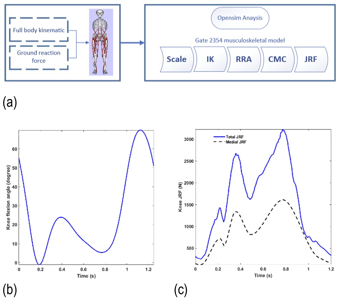
Fig. 6. Joint reaction force (JFR) analysis (a) OpenSim platform; (b) knee flexion angle; (c) total and medial joint reaction force
Initial Conditions and Model Setup
This section establishes initial conditions based on the static force solution applied to the femur. As shown in Fig. 7, the femoral reference point—corresponding to the primary Cartesian coordinates on the superior tibial surface—is positioned at an initial offset of 0.997 mm. The femoral profile was derived from potential cartilage contact regions identified through surface overlap analysis within the medial compartment. Due to the complex geometry of the femoral condyle, both penetration depth and contact trajectory were determined using a triangular mesh-based surface reconstruction algorithm applied to the three-dimensional knee model.
Simulations were performed over a complete gait cycle with a time step of 1×10⁻¹² s. For stiffness calculations, the contact geometry was modeled following reference [52], representing the articular surfaces as two spheres with radii of 34 mm (convex femoral surface) and 95 mm (concave tibial surface), respectively.
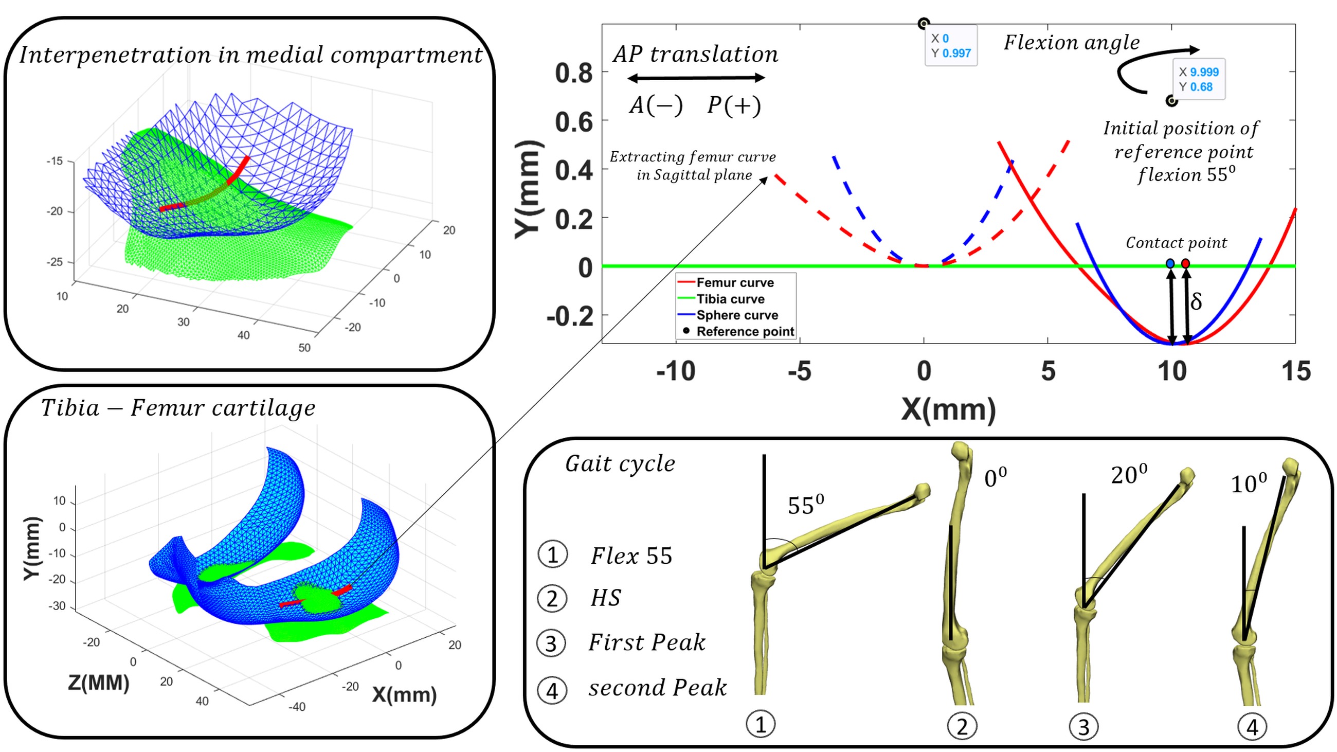
Fig. 7. Definition of the contact surface geometry (fitted curve) based on the overlapping region of the medial compartment of the tibiofemoral joint
Contact models play a crucial role in analyzing the dynamic behavior of mechanisms and in practical case studies [53-59]. Figure 8 presents the calculated knee contact forces using the Kelvin-Voigt contact model. This model was selected because Hertz-based models are inadequate for accurately describing soft material behavior [60]. The Kelvin-Voigt approach effectively simulates cartilage collision dynamics.
Figures 8 and 9a compare contact forces and penetration depths throughout the gait cycle between the sphere-plane model and the proposed fitted-curve-plane model. While both models show similar results in these figures, incorporating actual femoral geometry enables more accurate prediction of femoral dynamic behavior based on reference point motion. Figure 9b demonstrates the difference in femoral reference-point displacement in the y-direction, which is substantially larger than the variation observed in Figure 9a.
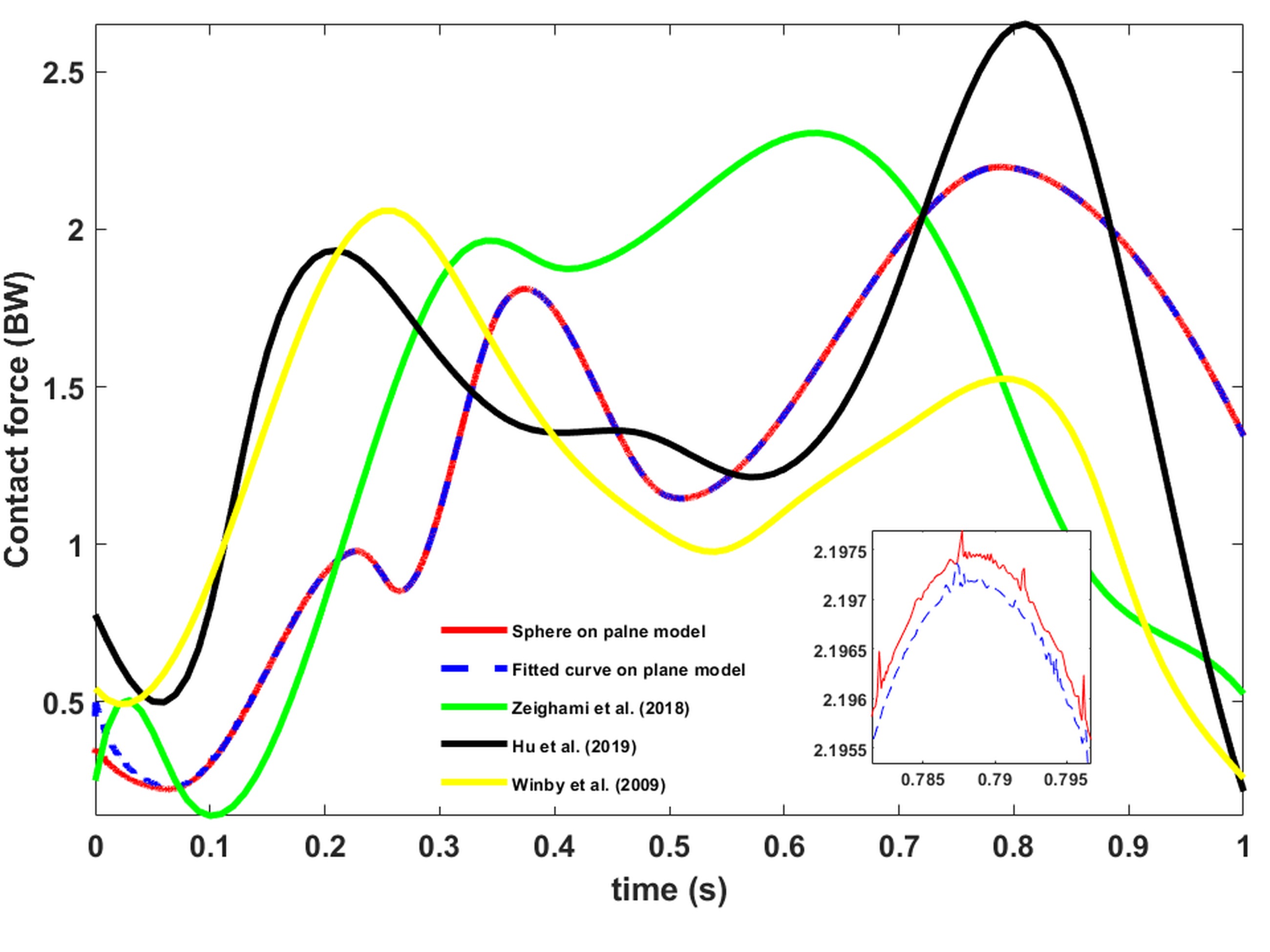
Fig. 8. Comparison of the medial knee joint contact force using the curve-fitting method for the femoral contact profile and the spherical femur model, along with validation against previous studies (BW: Body weight)
Figure 10 displays tibiofemoral joint contact points during the gait cycle. The contact points on tibial condyles at four gait phases align with findings reported in [38], as shown in Figure 11. Figure 11a illustrates contact points on the tibial plateau from an axial view, revealing anterior-posterior contact point migration. Figure 11b, derived from X-ray images in [38], shows good agreement with the contact-point pattern identified in this study.
Comparison between the curve-fitted and sphere-plane models reveals reduced cartilage penetration depth (δ) in the curve-fitted model, despite similar contact forces. Numerical results correspond to the second peak of contact force during the gait cycle. The curve-fitting approach yielded a cartilage penetration depth of 0.705 mm, representing a 0.6% reduction compared to the spherical model. As a key contribution, this study successfully integrates tibiofemoral cartilage penetration depth into biomechanical gait simulation. Figure 12 delineates medial tibiofemoral joint penetration depth and contact points during four critical gait phases: (a) 55° flexion, (b) heel-strike, (c) first peak, and (d) second peak, referenced to the anterior-posterior direction.
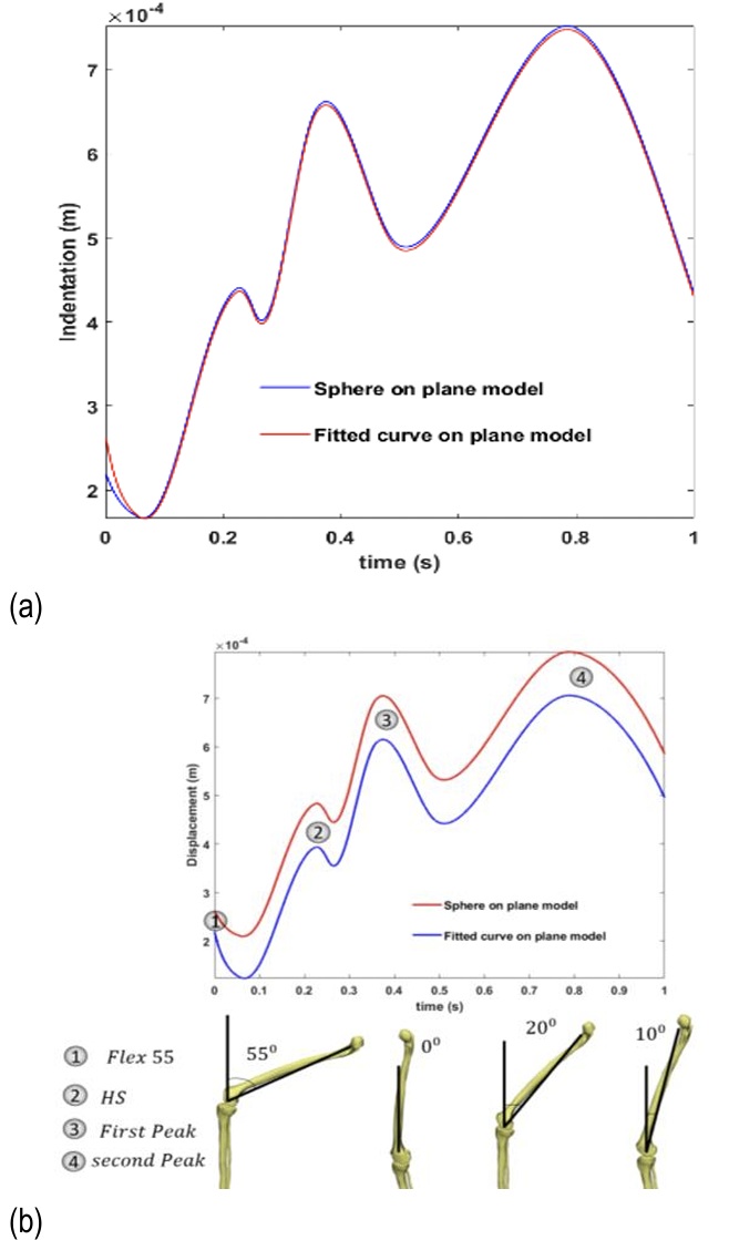
Fig. 9. Comparison of the curve-fitting method with the spherical femur model: (a) penetration depth in the medial knee joint, and (b) displacement in the y-direction
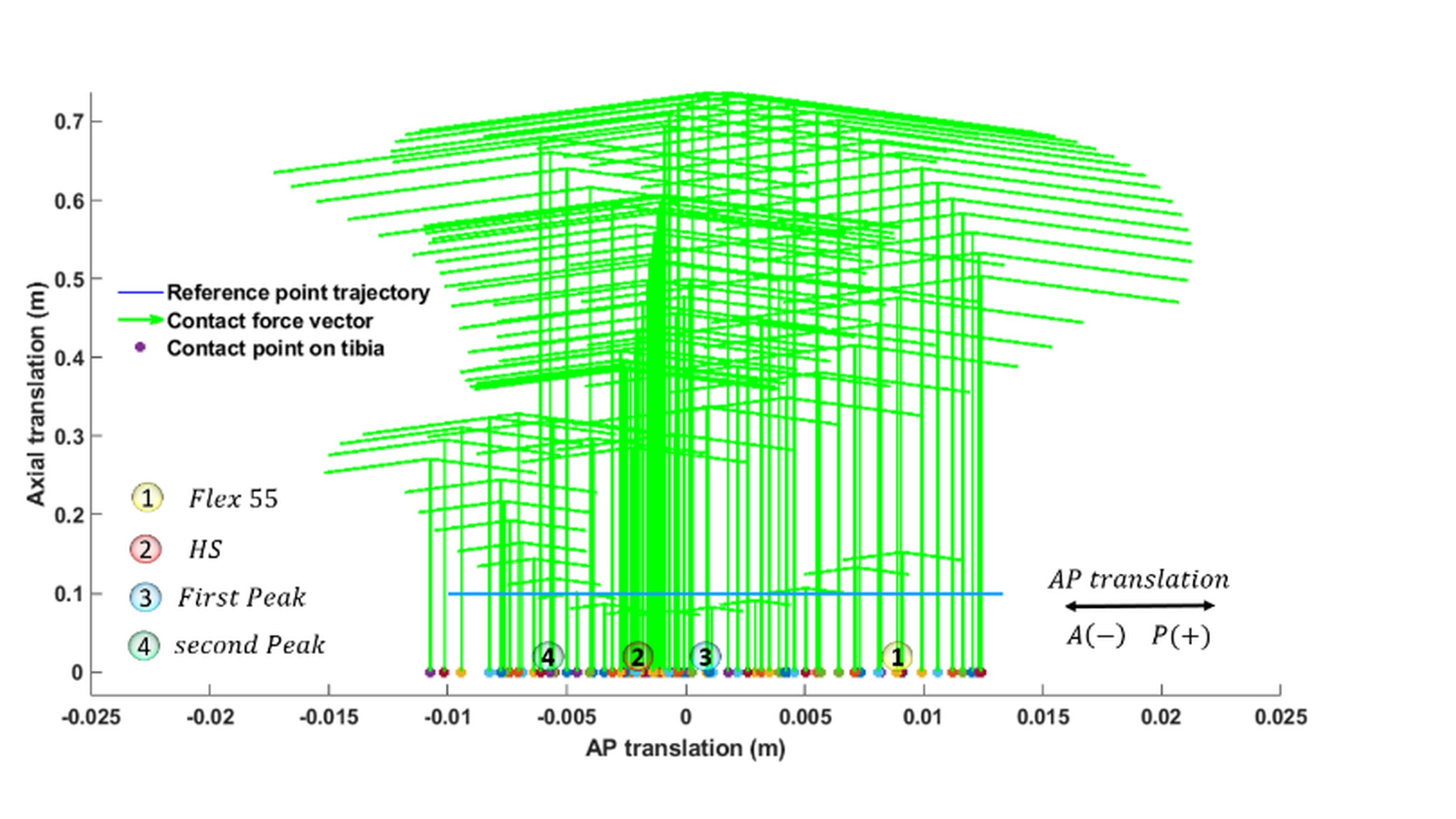
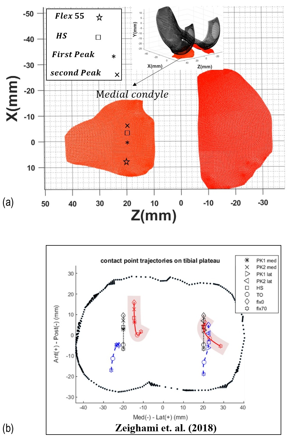
Fig. 11. (a) Knee joint response using the curve-fitting method: contact points in the axial plane; (b) experimental contact-point results obtained from X-ray images in the referenced literature
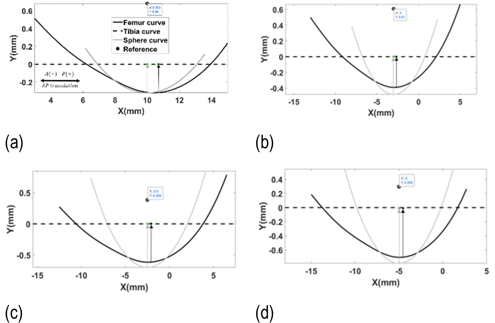
Fig. 12. Penetration depth and contact points of the medial tibiofemoral joint during the gait cycle: (a) 55° flexion angle; (b) heel-strike moment; (c) first peak; (d) second peak (AP: anterior–posterior direction)
In recent studies [61-62], healthy participants demonstrated distinct first and second peaks in the medial tibiofemoral contact force (FTN) during walking. The average magnitude of the first peak was approximately 1.8–2 body weight (BW), while the second peak averaged around 2–2.3 BW. Accordingly, the first and second peak values of the medial contact force as 1.81 BW and 2.19 BW, respectively, which are consistent with previously reported results [62-63]. Our model, which omits the menisci, provides an accurate prediction of cartilage penetration depth [30]. Similar to the findings in references [63-64], the exclusion of the meniscus does not cause a significant deviation in estimating the medial tibiofemoral contact force.
While our model omits the meniscus, similar to the approaches in [30-31, 64], it accurately predicts cartilage penetration depth. Therefore, although including the meniscus is preferable, it was omitted from our model—akin to the mentioned studies [30-31, 64] due to computational complexity and our specific focus on cartilage performance.
In-vivo imaging studies using combined dual-fluoroscopy and MRI have shown that peak tibiofemoral cartilage deformation during normal gait typically ranges between 7–23% of the resting cartilage thickness [65]. For a representative 3 mm cartilage layer, this corresponds to a maximum penetration of approximately 0.7 mm. MRI-based strain mapping studies have additionally reported regional compressive strains of 5-7% (≈0.15-0.21 mm for 3 mm thickness) [66], while higher deformations up to ~30% (≈0.9 mm) have been observed under more demanding loading conditions [67]. Therefore, the maximum penetration of ~0.7 mm reported in the present study is consistent with upper physiological values measured in healthy knees during gait.
The observed reduction in tibiofemoral contact force under OA conditions is a direct consequence of the penetration-based contact formulation, where decreased cartilage thickness reduces permissible penetration depth and thus contact force [53, 68]. This geometric effect is well-documented in computational studies using identical kinematic inputs [53, 68]. Importantly, this does not contradict clinical observations of elevated joint loading in OA patients, which is primarily driven by neuromuscular adaptations such as increased muscle co-contraction and altered gait patterns [69-70]. Our results specifically isolate the contact layers and geometric contribution, demonstrating that the documented clinical increase in load must stem from these compensatory neuromuscular mechanisms rather than the geometric changes themselves [69-70].
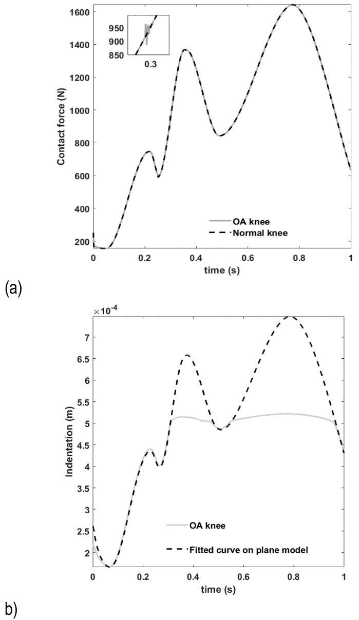
Fig. 13. Osteoarthritic knee joint response using the curve-fitting method: (a) contact force Fₜₙ, (b) penetration depth δ (Max BP: maximum net bone-on-bone penetration depth)
While the proposed two-dimensional knee model incorporates essential biomechanical features—including real-time computational capability, bone and cartilage representation, and medial condyle tibiofemoral contact force estimation—it excludes certain aspects of knee joint mechanics. Specifically, the current formulation does not account for abduction-adduction motion or the associated torque components in the frontal plane. Consequently, although the model effectively estimates net sagittal plane loads, it does not capture load transfer or torque interactions resulting from frontal-plane movements.
Although the model provides valuable biomechanical insights, it is not intended to replace detailed three-dimensional knee analyses required for clinical or diagnostic applications. Future developments should extend this framework toward a real-time capable 3D model that integrates frontal-plane dynamics while maintaining computational efficiency for human-machine interaction scenarios.
Further model enhancements could incorporate frontal-plane mechanics to establish correlations between medial/lateral compartment contact forces and abduction angles. In the current study, the cartilage-cartilage interface was modeled as frictionless, consistent with the extremely low friction coefficients reported for healthy, synovial-lubricated cartilage. Since novel friction models have not been adequately calibrated for knee joint conditions, accurate parameter estimation would require dedicated experimental or modeling studies. Implementing such knee-specific friction representations represents a promising direction for future research.
Conclusions
In conclusion, this study established a novel modeling workflow that integrates a customized knee joint model within the OpenSim musculoskeletal simulation framework to analyze knee kinematics and load distribution. The pipeline utilized inverse dynamics derived from motion capture and ground reaction force data to estimate joint reaction and cartilage contact forces.
A two-dimensional knee model with MRI-derived geometry was developed and simulated using a forward dynamics approach. Reflecting the clinical importance of contact mechanics in osteoarthritic joints, the analysis focused on quantifying indentation and contact patterns, including cartilage-on-cartilage and bone-on-bone interactions. A computational method was formulated to calculate penetration depth for complex, curved surfaces against a planar contact surface.
To evaluate the sensitivity of contact mechanics to geometrical representation, the anatomically-based fitted-curve model was systematically compared against a simplified spherical model. This comparison demonstrated that while both models capture general trends in contact forces and penetration depth, the anatomical fitting provides superior accuracy in predicting localized contact patterns and femoral trajectory.
Simulation results revealed distinct variations in contact forces and cartilage indentation between healthy and osteoarthritic knee models. The osteoarthritic configuration exhibited reduced indentation and lower contact forces, attributable to the altered mechanical environment and increased bone-on-bone contact stiffness. The model outputs showed strong agreement with established biomechanical data in the literature, validating the approach. Force distribution across the tibial plateau was analyzed using dynamic knee MRI data.
This integrated OpenSim-based approach successfully quantifies critical biomechanical parameters—including contact points, indentation, and contact forces—providing a valuable tool for assistive device design, surgical planning, and further investigation of knee joint biomechanics.