
. INTRODUCTION
Although the problem of vertical vehicle vibration has received considerable attention in extensive literature [1-5], it mainly concerns partial solutions of simple half models with a longitudinal axis of symmetry, i.e., a system with two degrees of freedom, which, however, does not describe vehicle behavior with sufficient accuracy. These models address the effects of shifting the center of gravity from the center of the axle spacing or different suspension stiffnesses, possibly with different damping intensities, or combinations thereof. Most often, vehicle model vibration problems are solved using so-called quarter models, usually with a varying number of bodies, vertically flexibly connected and with dissipative elements, i.e., models with multiple degrees of freedom with connected vertical displacements. The application of a quarter model assumes two axes of symmetry of the vehicle, i.e., complete symmetry of the vehicle and its kinematic excitation. None of the above models corresponds to reality, and these solutions do not provide a sufficiently accurate picture of the vehicle's behavior, so it is important to address these issues on a complete spatial model of the vehicles.
Another approximation is a three-dimensional model, i.e., a spatially flexible body with two, three, or generally up to six degrees of freedom, or a system of two or more bodies defined by mass and moments of inertia with six or more degrees of freedom (e.g., a locomotive model with up to 270° of freedom [6]), possibly again taking energy dissipation into account. However, there is no solution for the influence of asymmetry in spatial vehicle models.
When analyzing the influence of vehicle model asymmetry on its vertical vibration, it is necessary to distinguish between three basic cases of asymmetry with respect to the axes of geometric symmetry [6], which are determined by two mutually perpendicular axes of symmetry, the track and wheelbase of the vehicle, and intersect at the geometric center of the vehicle.
1.asymmetry of vehicle weight distribution relative to the axes of geometric symmetry, position of the center of gravity, directions of the main central axes of inertia of both the vehicle structure itself and the loaded vehicle
2.asymmetry in the geometry of the distribution of elastic and dissipative elements of the connections between individual bodies of the vehicle system and their mechanical properties, spring stiffness, viscous damping intensity, assuming linear connections between individual variables and small displacements and rotations of parts of the system
3.asymmetry of kinematic excitation, i.e., the field of unevenness of the road surface or rails, defining the kinematic excitation of the system at the point of contact between the wheel and the road surface or between the wheel and the rail.
These types of asymmetry can exist separately or together. Most often, practically always, the third case occurs.
. METHODOLOGY
The basic prerequisite for investigating the influence of asymmetry was the selection of a suitable simple spatial model for investigating various cases of asymmetry with the possibility of comparing and verifying the results obtained by different methods – experimental and theoretical (analytical, numerical, and simulation). - the time course of various investigated variables, e.g., vertical displacement of the center of gravity w and rotation φx, φy around axes passing through the center of gravity, and especially the vertical displacement over time of any point of the vehicle model – mechanical system.
For the analytical solution of vertical vibration of the vehicle model, Lagrange equations were used to derive the equations of motion of a flexibly mounted body, or a system of bodies mounted and connected by flexible and dissipative elements, under the influence of kinematic excitation of the system when crossing obstacles. The equations of motion were solved by applying Laplace transformation. During the inverse transformation, the resulting motion was decomposed by summing the convolution integrals of the individual components of motion with the corresponding natural frequency, i.e., the motion caused by the individual components of the kinematic excitation function vector [6].
The simplest general spatial model can be implemented as a rigid plate mounted on springs, kinematically excited by unit jumps (Fig. 1). This model can be easily used to implement various kinematic excitations (by combining the jumps of individual springs) as well as structural and load asymmetry using various weights (counterweights) placed at different points on the upper surface. This shifts the position of the center of gravity from the geometric center C to the center of gravity of the model T.
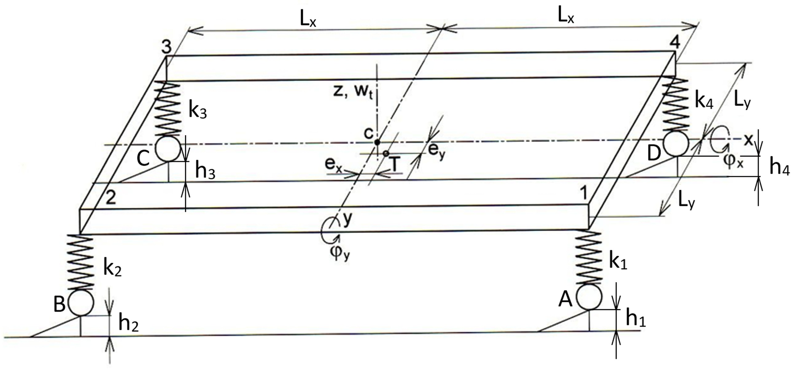
Fig. 1. Basic scheme of the model: e y, e x – eccentricity, w t – vertical displacement, h i – height of the jump of the i -th spring (i = 1, 2, 3, 4), A, B, C, D – wheel designation, φ x, φ y – rotations, c – geometric centre, T – center of gravity, L x, L y – distance of wheels from the center of gravity in the x and y axes.
In this general spatial model, the resulting time vertical displacement of any point i is given by the relationship:

The equations of motion of the adopted model can be written in general matrix form from Lagrange's equations of the second kind.

where: M – mass matrix, which includes the weight of the plate (vehicle), moments of inertia in the x and y axes, and deviation moments in the xy and yx planes , B – damping matrix, K = (aik) – stifness matrix, aik - stiffness matrix elements, which are functions of the dimension li, spring stiffness ki and eccentricities ex, ey, qj(t) - generalized coordinate vector (qj(t) => z(t),φx(t), φy(t)), Fj(t) - vector of the excitation function (Fj(t) => Fz(t), Fx(t), Fy(t)).
The given system of ordinary differential non-homogeneous equations is solved analytically by applying Laplace integral transformation. After transforming the system of differential equations, a system of algebraic equations is obtained:

where: qj(p),F(p) – function vector images qj(t) a Fj(t).
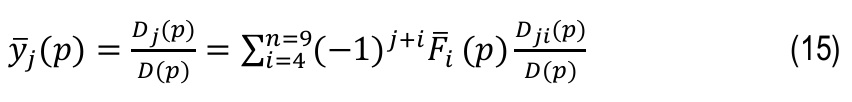
The solution to system (3) can be written as:

where: D(p) - determinant of the matrix D(p), determinant Dj(p) arises from the determinant D(p) by replacing elements of the j-th column with elements of the vector Fj(p), Dji(p) - algebraic complement of the determinant Dj(p).
For the inverse transformation, it is necessary to solve a frequency algebraic equation of degree n = 2p, i.e., twice the number of degrees of freedom of the system, which is the most complicated part of the entire solution. Therefore, a method [8] was proposed that meets the requirements for analyzing the vibration of mechanical systems with a lower number of degrees of freedom, approximately p = 10.
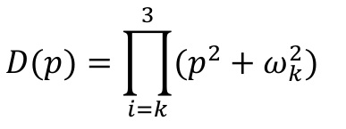
For the inverse transformation, it is advisable to adjust the ratio of determinants in relation (4) to a form that allows the application of the convolution theorem. The characteristic polynomial of the determinant D(p) can be adjusted to the form of the product of root factors [6]:
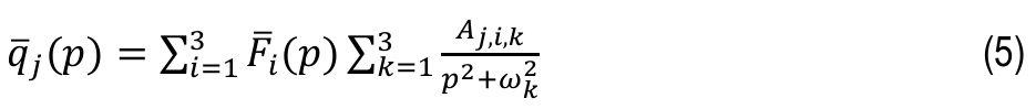
and obtain the desired solution by converting the ratio of determinants in relation (4) to the sum of partial fractions using the method of indeterminate coefficients (Aj,i,k).
This procedure yields the solution to system (3) in the form:
where the coefficients Aj,i,k are functions of the elements of the weight and stiffness matrices [8]. After reverse transformation and adjustment, the solution to system (2) can be written in the form using the input variables
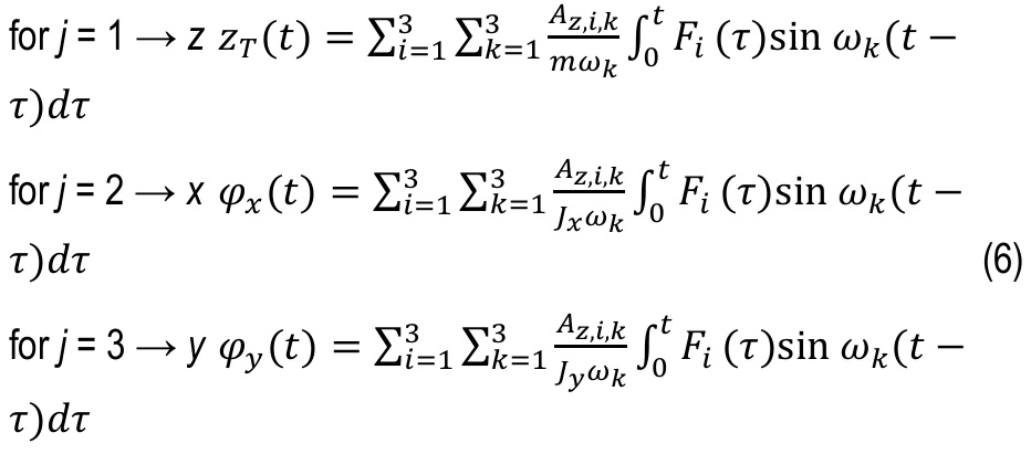
The sought coordinates zT(t), φx(t), φy(t) are determined in the case of asymmetry by the sum of nine convolution integrals. The vertical displacement of any point on the plate – a rigid body – can be determined using relations (1) and (6). Neglecting the influence of unsprung masses, the time course of the vertical dynamic component of the contact force between the wheel and the rigid base (road, rail) can be expressed in the form of the simplest vehicle model as follows:

where index i determines the location of the elastic mounting, hi(t) – height of the i-th spring jump depending on time t. The resulting vertical component of the contact force is given by the superposition of the dynamic Rdi(t) and static component Rsi = wsi·ki.
In a symmetrical arrangement of the system, both the mass matrix (Dxy = 0) and the stiffness matrix (aij = 0 for i ≠ j) are diagonal. System (2) or (3) changes to three mutually independent equations. Their solution can be written in the form:
A comparison of relations (6) and (7) indicates the influence of asymmetry in the oscillation of the system. The assessment of the influence of asymmetry for a specific system will be possible after numerical quantification and comparison of the time course of the variables zT(t), φx(t), φy(t) according to relations (6) and (7) and, above all, by comparing the resulting time course of the vertical displacement at any point according to relations (1), (6) and (7) in both cases.
. SOLUTION
The above method was first used to solve a simple vehicle model (Fig. 1) with three degrees of freedom, without damping, with asymmetry caused by the eccentric position of the center of gravity ex, ey from the axis of geometric symmetry, with symmetrical kinematic excitation by simultaneous jumping of all wheels from wedges of unit height h. Evaluation of previously derived relationships, e.g., for calculating the vertical displacement of the center of gravity zT(t) – see Figs. 2 and 3.
The significance of asymmetry's influence on vehicle vibration is particularly evident when investigating vertical displacements at the point of flexible mounting of the plate – the vehicle. Vertical displacement at a general point on the plate is given by equation (1). Then vertical displacements at points 1 to 4.
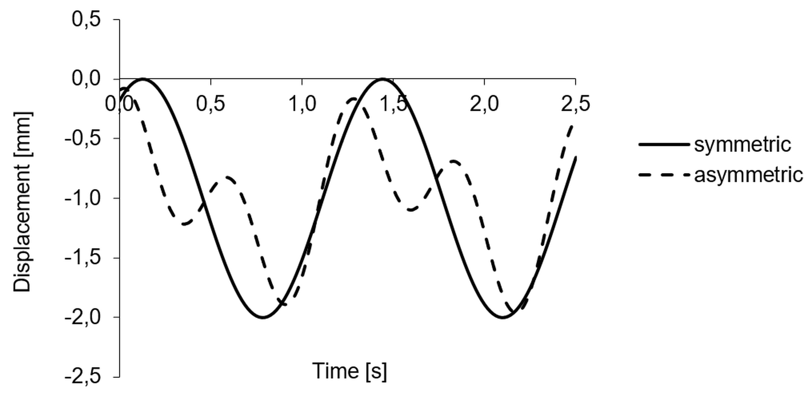
Fig. 2. Vertical displacement of the centre of gravity in symmetrical and asymmetrical wedge jump - without damping - analytical solution
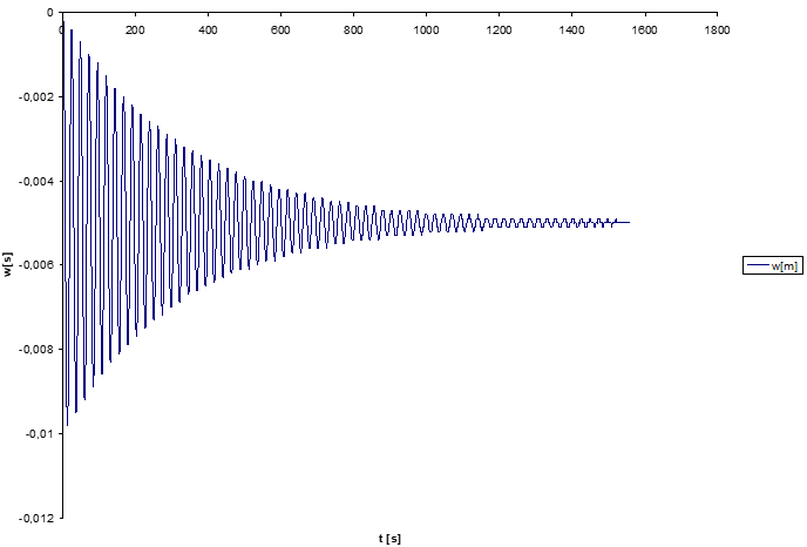
Fig. 3. Oscillation of the centre of gravity of the system under symmetrical loading and excitation of the system - experiment
The time change in vertical displacements at the flexible mounting points 1 to 4 corresponds to the time change in wheel pressures of the vehicle (A, B, C, D). Fig. 4 shows the displacement curve of point 1 in the case of a symmetrical model that was excited symmetrically w1A-D (drop of all 4 wheels, A-D) and asymmetrically w1A (drop of wheel A), w1B (drop of wheel B), w1C (drop of wheel C), w1D (drop of wheel D).
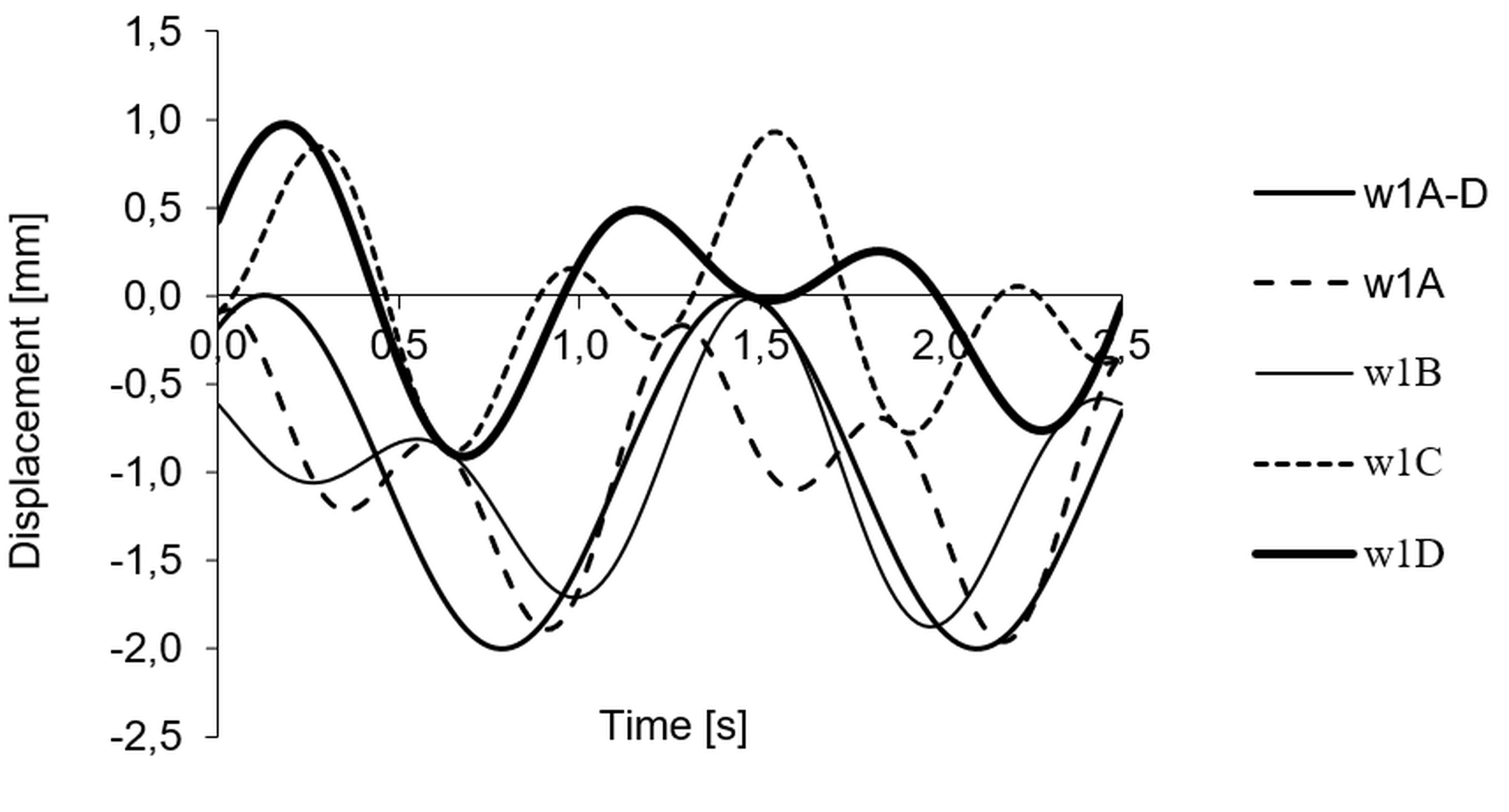
Fig. 4. Symmetric model symmetrically (w 1 A-D) and differently asymmetrically (w 1 A, w 1 B, w 1 C and w 1D) excited and measured at point 1
As part of the solution for vertical vibration, more complex models were also developed for both railway and road vehicles. Here we present an outline of the solution for a two-axle railway vehicle and a bogie vehicle.
To investigate vertical displacements of a two-axle rail vehicle, under certain assumptions, it is possible to choose a rigid rectangular plate with asymmetrically distributed mass relative to the geometric axes of symmetry of the centerline surface, spatially flexibly mounted on four coil springs, as a calculation model. The investigation of vertical displacements of the plate for various cases of asymmetry during kinematic excitation of a system with three degrees of freedom, corresponding to the vertical displacement of the center of gravity w, rotation φx and φy around the central axes of inertia of the plate, has been presented in several papers, e.g., [6].
Vertical displacements are investigated for a model of a two-axle vehicle, or a rigid plate with the influence of energy dissipation during oscillatory movements. The flexible mounting of the plate is combined with a parallel viscous damper (Fig. 5).
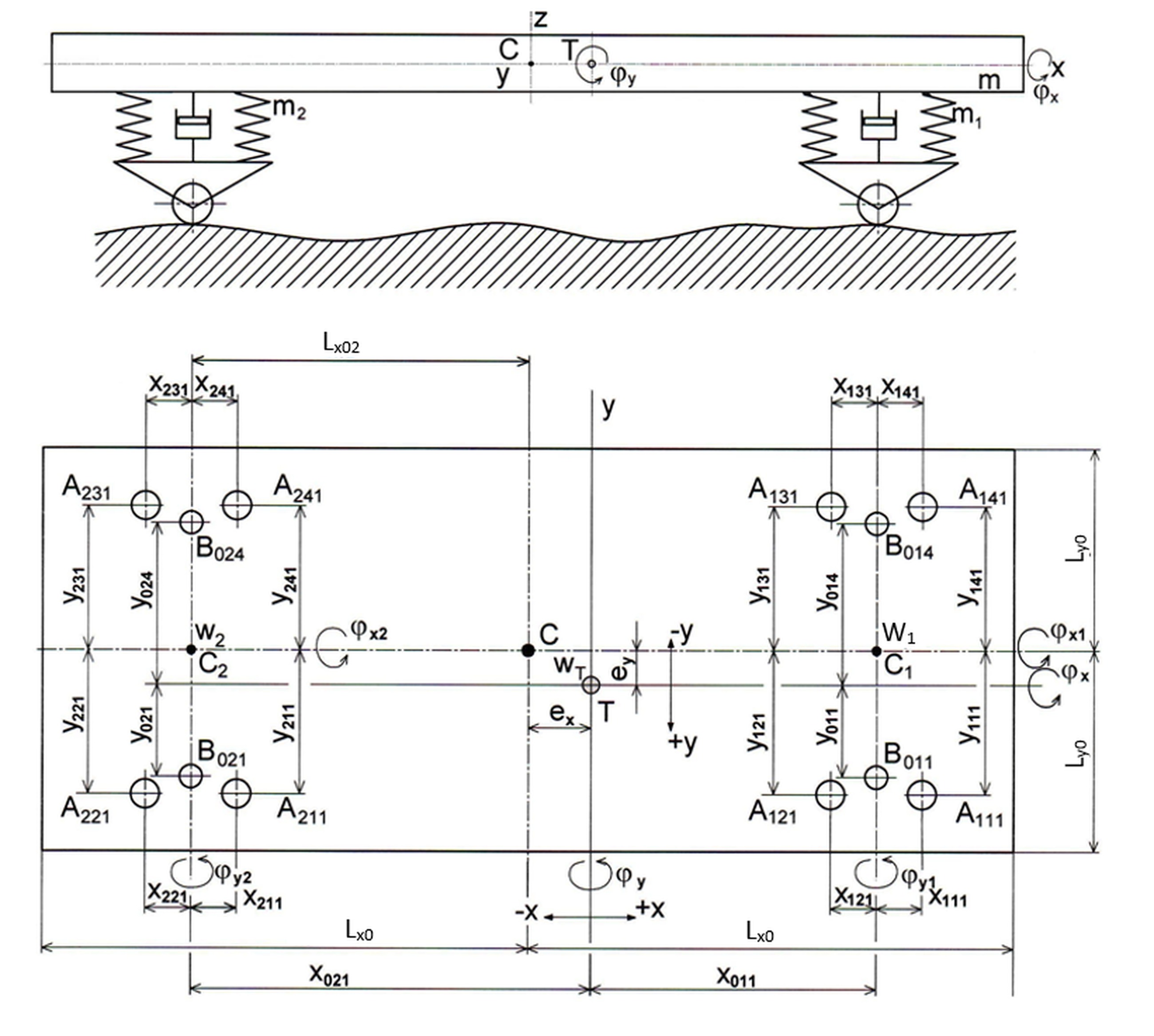
Fig. 5. Double-axle vehicle with damping: c - geometric centre of enclosure, e x, e y – eccentricity, m – weight of enclosure B, m 1,2 – weight of chassis A, w T – vertical displacement, x, y, z – axes, x jki, y jki – coordinates of points A and B. A jki – point on chassis (j = 1, 2 – number of chassis, k = 1, 2, 3, 4 – number of quadrant, i = 1, …, n – sequence of spring), B jki – point on enclosure (j = 0 – only one enclosure, k = 1, 2, 3, 4 – number of quadrant, i = 1, …, n – sequence of spring), L x, L y – distance of springs from the center of gravity in the x and y axes, T - center of gravity, φ x, φ y – rotation around the x and y axes.
In the case of spatial storage of the plate, the equations of motion can be written in matrix form:
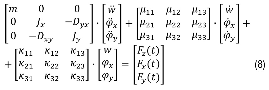
Jx, Jy – moments of inertia, Dxy, Dyx – deviation moments to the central axes of the plate, Fz(t), Fx(t), Fy(t) – functions of external excitation, including kinematic load.
The system of equations (8) can be modified to the form
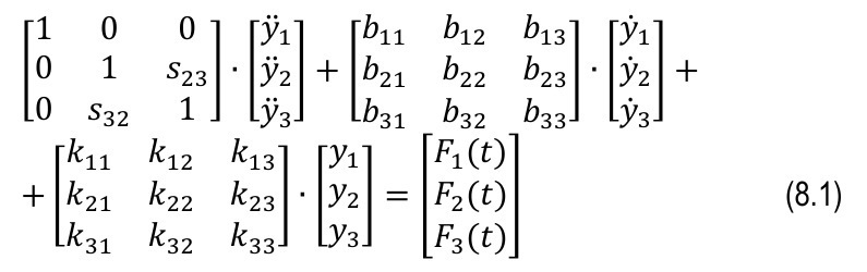
where the elements of the mass matrix s23 = -Dyx/Jx, s32 = -Dxy/Jy determine the effect of the asymmetry of the mass distribution, or rotation of the principal axes of inertia relative to the central axes of inertia.
The solution was performed by applying Laplace's transform, assuming zero initial conditions, and the resulting system of linear algebraic equations was solved using Cramer's rule.
A detailed mathematical solution to this problem, including the calculation of coefficients, is given, for example, in [6]. Given the general formulation of the task presented here, the calculation of the oscillation, i.e., the vertical displacement of a general point of a body with a generally distributed mass, spatially generally mounted on vertical springs and hydraulic shock absorbers, which is caused by the excitation function of a general time course, can be performed using known procedures. Therefore, we do not deal with a detailed solution here (a number of computational procedures can be used, e.g., in MAPLE, MATLAB etc., or even numerical methods for calculating systems of second-order differential equations, e.g., Newmark or Runge-Kuth etc.).
Another model solved was a kinematically excited system of three spatially flexibly mounted and connected bodies. This problem was solved by selecting a railway bogie model (Fig. 6) with 9 degrees of freedom.
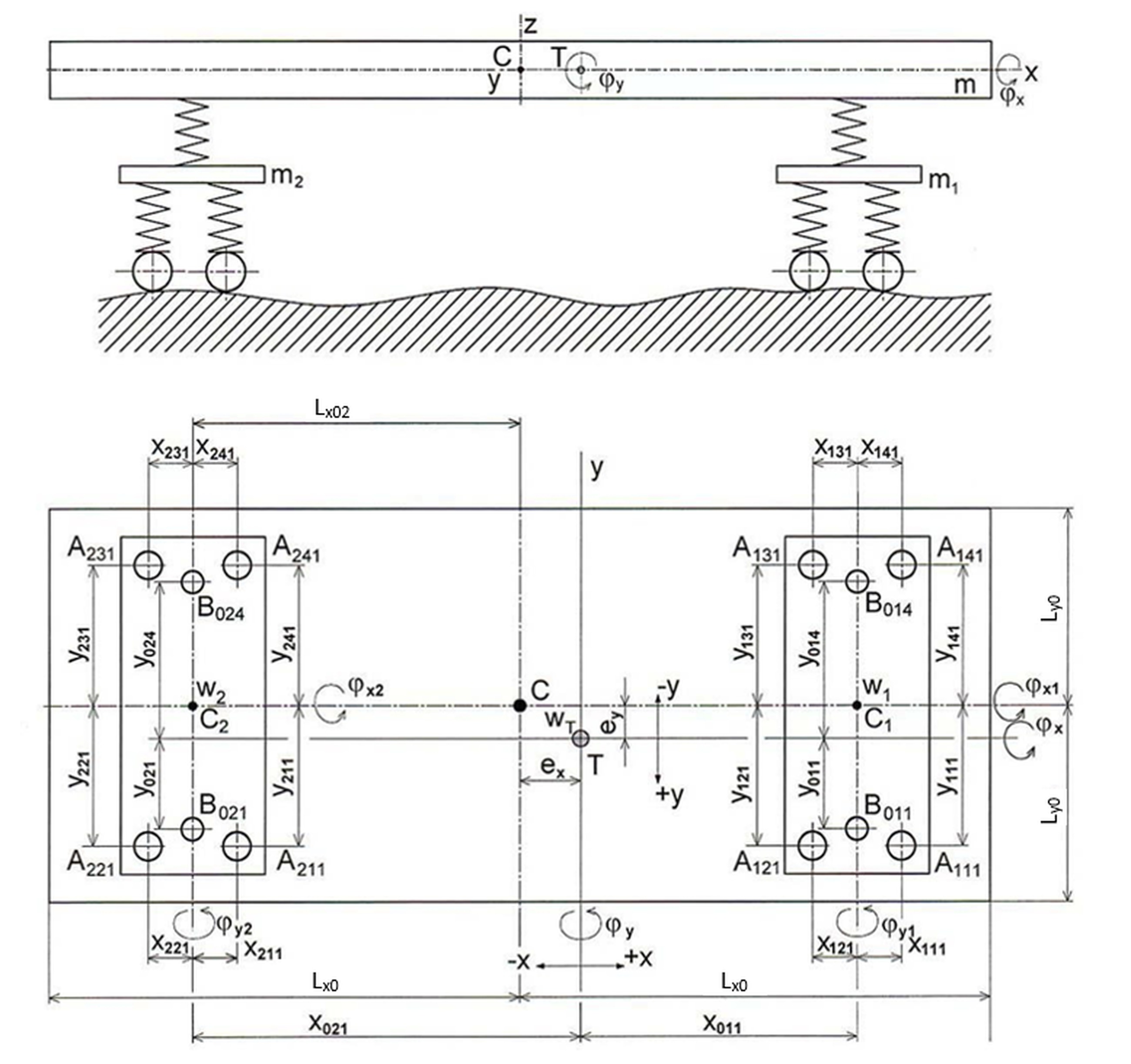
Fig. 6. Model of a rail bogie wagon: c - geometric centre of enclosure, e x, e y – eccentricity, m –weight of enclosure B, m 1,2 – weight of chassis A w T – vertical displacement, x, y, z – axes, x jki, y jki – coordinates of points A and B. A jki – point on chassis (j = 1, 2 – number of chassis, k = 1, 2, 3, 4 – number of quadrant, i = 1, …, n – sequence of spring), B jki – point on enclosure (j = 0 – only one enclosure, k = 1, 2, 3, 4 – number of quadrant, i = 1, …, n – sequence of spring), L x, L y – distance of springs from the center of gravity in the x and y axes, T – center of gravity, φ x, φ y – rotation around the x and y axes.
The equations of motion of a kinematically excited system of three rigid bodies spatially flexibly mounted and connected as a model of a rail vehicle chassis with primary and secondary linear suspension, taking into account the effect of asymmetry, were derived. The solution of problems in the dynamics of road and rail vehicles based on various assumptions and under various conditions has long been the subject of considerable attention, which is why this solution is the subject of extensive technical literature, e.g., [1, 2, 7] and others. However, the influence of asymmetry has not been addressed.
The simplest computational model of a vehicle chassis, see Fig. 6, consists of two-axle chassis with simple primary suspension and simple vehicle body suspension. For chassis models – rigid plates with masses m1 and m2 – symmetry of mass distribution is considered, i.e., the position of the center of gravity is identical to the geometric center, and the main central axes of inertia are identical to the axes of geometric symmetry. The asymmetry of spring stiffness parameters and their geometric mounting is considered.
For the vehicle body model and rigid plate with mass m, an asymmetrical mass distribution is considered, i.e., the position of the center of gravity is deflected by ex and ey from the geometric center, and the main central axes of inertia are rotated relative to the axes of geometric symmetry. Differences in the stiffness parameters and geometry of the secondary suspension mounting are considered.
The solution is based on general assumptions, i.e., the stiffness of bodies, small displacements and rotations, linear characteristics of springs, and further assuming that only the vertical displacement of any point of individual bodies is considered, i.e., the vertical change in position of any point of the body, which is determined by the displacement of the center of gravity of the body w, w1, w2 and the displacement of the point resulting from the rotation φx and φy, φx1 and φy1, φx2 and φy2 around the central axes of inertia of individual masses m, m1, m2 and its distance from these axes. It is therefore a system of bodies with nine degrees of freedom.
The equations of motion are derived using Lagrange equations of the second kind. Therefore, it is necessary to determine the kinetic energy Ek and potential energy Ep of the oscillating system.
Kinetic energy of the system:
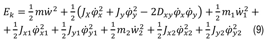
where: Jx, Jy – moments of inertia, Dxy – deviation moment to the central axes of inertia of the body with mass m, Jx1 and Jy1, resp. Jx2 and Jy2 – moments of inertia to the main central axes of inertia of the chassis with mass m1, resp. m2.
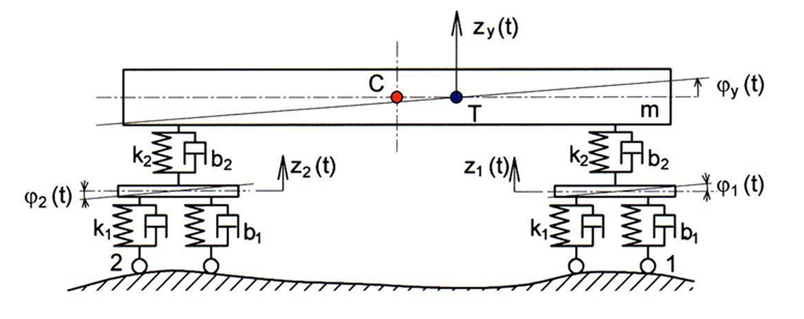
Fig. 7. Suspension specification: c – geometric centre of enclosure, m –weight, z y (t) – displacement in the z -axis depending on time t, z 1,2 (t) – displacement of chassis 1, 2 depending on time t, k 1 – stiffness of primary suspension springs, k 2 – stiffness of secondary suspension springs, b 1 – primary suspension damping, b 2 – secondary suspension damping, φ y – rotation around the y -axis, T – center of gravity, φ 1 – rotation of the first chassis, φ 2 – rotation of the second chassis, 1 – first chassis, 2 – second chassis
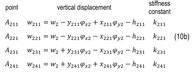
To determine the potential energy, it is necessary to determine the displacements of individual masses at the point of their elastic mounting (see Fig. 6 and Fig. 7). The displacements of individual points of the chassis are given by the following relationships:
Body m1, j = 1
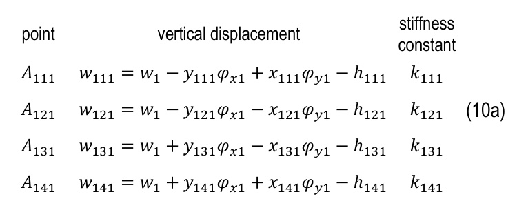
where the system corresponds to the designation of points Ajki, their coordinates xjki, yjki, vertical displacements wjki, and spring stiffness constants kjki for masses j = 1, 2, quadrants k = 1, 2, 3, 4, and spring order i = 1, … n - for multiple mounting. Similarly, the vertical change hjki is marked at the point of spring mounting in the rigid base to which the position of the body relates.
Body m2, j = 2
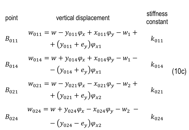
In the case of a enclosure model with simple suspension using a single spring in the axis of the relevant chassis, it is not possible to use a division into quadrants to designate the individual points of action of the springs. The designation of points, coordinates, and stiffness constants Bjki, xjki, yjki, kjki, j = 0 body, mass m, k = 1, 2 designation of the respective chassis 1 or 2, i = 1, 4 affiliation to half of point A111 or A141 is shown in Fig. 6.
The displacements of the individual points of the body are given by the following relationships:
The potential energy of the chassis models m1 and m2 and the enclosure model m is:
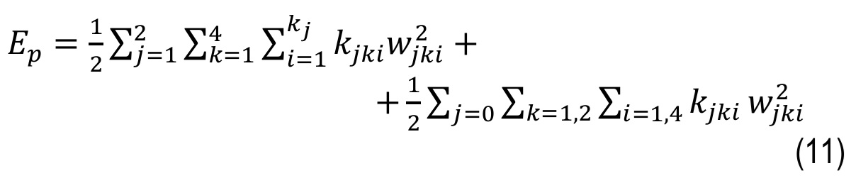
We substitute the displacements (10a, b, c) into equation (11) and substitute the modified equation for potential energy Ep together with kinetic energy Ek from equation (9) into the Lagrange equations of the second kind.
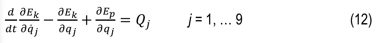
where the generalized coordinates qj = (φx, φy, w, w1, w2, φx1, φy1, φx2, φy2)T and Qj are generalized forces, including kinematic excitation. After performing the relevant derivations according to individual coordinates, the equations of motion are obtained in matrix form (13).
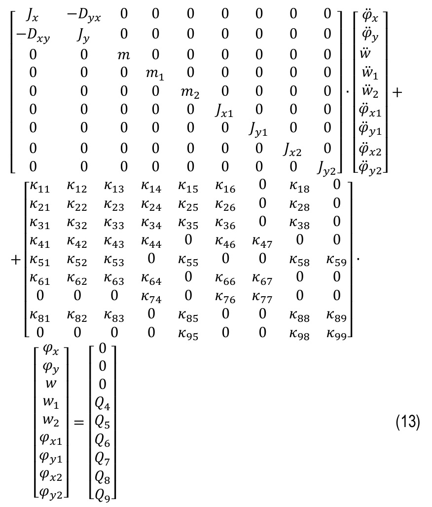
where the individual elements of the stiffness matrix κij are functions of the stiffness constants kjki and the dimensions of the mounting geometry xjki, yjki, and the eccentricities ex and ey – Fig. 6. The calculation of the coefficients κij and the excitation forces Qi is given in [6].
For further solutions, for a general formulation of its procedure and the creation of a suitable algorithm for computer processing of the generalized solution, system (13) is modified to the form:

The solution to the system of non-homogeneous differential equations (14) can be obtained using one of the numerical methods; the analytical solution can be performed by applying matrix calculus or the Lagrange method of variation of constants or by applying the Laplace transform. Using this method, after transformation, a system of linear algebraic equations is obtained for zero initial conditions [6].
The solution of the system of linear algebraic equations obtained is best performed using Cramer's rule:
where: D(p) – determinant of the matrix of the system of algebraic equations and is equal to:

For real coefficients A2(n-i), relationships were derived in [6] that generally apply for n ≥ 2 and 0 ≤ i < n. The formulas for calculating the coefficients A2(n-i) for 2 < i < n are very complex and confusing. The MAPLE or MATLAB software systems can be used to calculate the values of these coefficients.
By solving the above equations, after determining the coefficients of the algebraic equation and its root factors, we obtain an algebraic equation and a frequency equation in the form:
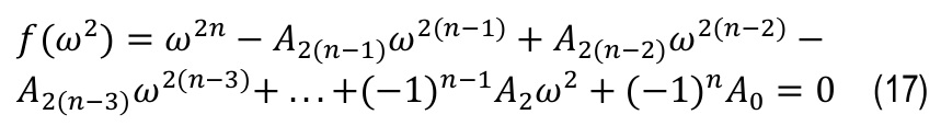
Determining the roots of the frequency equation (17) using a suitable numerical method is the most complicated part of the proposed solution, not only in terms of numerical accuracy, i.e., ω2 – circular frequencies of functions yj(t), for j = 1, 2, 3, …, n – solving a system of algebraic equations. Another solution and transformation.
After reverse transformation, the convolution integral is obtained
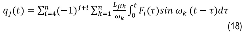
where ωk is the solution to equation (17). From the known functions qj(t), i.e., the solution to the system of equations (14), the sought quantities of the system of equations (13) are determined.
This makes it possible to determine the vertical displacements of arbitrary points of the chassis or enclosure, e.g., the displacements of the points described by equations (10a), (10b), and (10c).
. CONCLUSION
The article briefly summarizes findings from the solution of a system of rigid bodies flexibly connected. It outlines the issue of application to the solution of vertical vibration of vehicles, both road and rail. To date, relatively little attention has been paid to the vertical vibration of vehicles under asymmetrical loading and asymmetrical kinematic excitation of vertical vibrations.
Inappropriate asymmetrical loading, combined with kinematic excitation (e.g., a depression in the road surface, an obstacle (stone) on the rail), can lead to a loss of stability due to vehicle oscillation and loss of wheel contact with the road surface (rail). Inappropriate asymmetrical weight distribution leads to uneven loading of individual bogies, both longitudinally and transversely. The same problem occurs in road vehicles, where asymmetrical loading also leads to different loads on individual axles. This asymmetrical loading causes some axles to be relieved, and as a result of asymmetrical kinematic excitation, the axle may be completely relieved and lose contact with the road surface. In road vehicles, this phenomenon occurs mainly on the front axle, where the lightening of one or both steerable wheels causes a loss of contact with the road surface and thus the uncontrollability of the vehicle. In rail vehicles, this can result in a large vertical displacement at the contact point between the wheel and the rail, leading to derailment. It is therefore clear that particular attention must be paid to the correct distribution of weight (load), especially in trucks. In rail vehicles, it is important to ensure that the load is evenly distributed between both bogies, while in road vehicles, the requirement for correct loading of the steerable (usually front) axle must also be taken into account. The solution outlined in the article allows us to assess the correctness of the weight distribution and thus the load on individual bogies (and axles) so that this situation does not occur during asymmetrical kinematic excitation. To resolve this situation, it is appropriate to use the simple models discussed, which can be used to deduce when contact with the track will be lost and thus adjust the weight distribution, damping constants, and stiffness constants.
Loss of contact between the wheel and the track is probably the cause of "inexplicable" accidents. None of these aspects are addressed today by even extensive simulation methods and FEM; it is necessary to understand the physical essence and describe it analytically.
The proposed solution enables the creation of a program for calculating vertical displacements at any points of the model of rail vehicles with a wide range of specific design configurations.