INTRODUCTION
Flow boiling in minichannels
Flow boiling in minichannels has attracted significant attention over the past three decades due to its high heat removal capability and compactness, which are essential for modern thermal management systems in electronics cooling, energy systems, and process engineering. The combination of large heat transfer surface-to-volume ratios and enhanced convective and phase-change mechanisms allows minichannel heat exchangers to achieve high thermal performance while maintaining relatively small footprints. However, these advantages are often accompanied by increased flow resistance and susceptibility to hydrodynamic and thermal instabilities, which can limit practical applications.
The following presents a brief review of experimental studies addressing heat transfer and flow resistance in refrigerant flow through heat exchangers with minichannels.
The experimental studies discussed in [1] focused on heat transfer and pressure drop during flow boiling of the R134a refrigerant in microchannels with diameters of 0.5 mm and 1 mm. It was shown that the heat transfer coefficient (HTC) strongly depends on the heat flux but is practically independent of mass velocity. The maximum increase in the average heat transfer coefficient, amounting to approximately 22%, was achieved in the smaller channel. The pressure drop in the microchannels increased with increasing mass velocity and was also higher for smaller channel diameters.
In [2], it was observed that heat transfer enhancement achieved by mechanical modification of the heat transfer surface with cross-cuts leads to a change in the trend of the HTC curve and a reduction in flow resistance of about 25%.
In [3], the flow resistance and heat transfer characteristics of a copper microchannel heat sink cooled with deionized water were investigated at two heat flux levels. It was found that higher Reynolds numbers improve cooling efficiency (lower outlet and internal temperatures) but result in a higher flow resistance.
In [4], the authors experimentally analysed the effect of minichannel geometry on pressure drop and HTCs during the flow of air and water through minichannels with smooth walls and with attached circular ribs. The use of ribs significantly increased both pressure drop and heat transfer efficiency. An increase in the Reynolds number simultaneously resulted in an increase in pressure drop and improved thermal performance. Accurate characterization of pressure drop and heat transfer during flow boiling in minichannels remains challenging.
Analysis of the results presented in [1–4] showed that heat transfer efficiency in micro- and minichannels strongly depends on their geometry, heat flux, and Reynolds number. Increasing thermal efficiency is often associated with an increase in pressure drop and other undesirable phenomena, such as: uneven temperature profiles across the exchanger surface, uneven flow and phase distributions (in multiphase flows), local overheating, and minichannel blocking.
The interaction between liquid and vapor phases leads to complex flow patterns, strongly coupled momentum and energy transport, and time-dependent fluctuations of pressure and temperature. These effects are particularly pronounced in channels with hydraulic diameters on the order of millimetres or below, where surface tension, confinement, and local heat flux nonuniformities play a dominant role. As a result, correlations and models developed for conventional channels are often not directly applicable to minichannel configurations, necessitating dedicated experimental and analytical studies.
Trefftz and inverse heat transfer methods
From the modelling perspective, inverse heat transfer problems associated with boiling flows remain challenging due to their ill-posed character and sensitivity to experimental data. In the present study, the inverse formulation is coupled with experimentally measured thermal and flow parameters, which serve as boundary-condition data and reference values for validation of the reconstructed temperature fields.
From an engineering modelling perspective, a direct problem is defined by a governing equation, appropriate initial and boundary conditions, material properties, and geometric characteristics. When one or more of these elements are unknown, the problem becomes an inverse problem. Inverse problems are inherently ill-posed and highly sensitive to input data, often resulting in unstable solutions [5]. Therefore, numerical methods applied to such problems must emphasize stability and accuracy. Methods based on Trefftz functions are particularly well suited for this purpose [6,7].
In the Trefftz function approaches, the governing differential equation is satisfied exactly, while boundary and initial conditions are approximated. From a numerical standpoint, the Trefftz functions method offers a distinct advantage: it requires minimization of an (n−1)-dimensional integral for an n-dimensional differential equation, while e.g. the Ritz method requires minimization of an n-dimensional integral [7].
The dynamic development of the Trefftz method began in the 1970s, with significant contributions from Herrera, Jirousek, Sabina, and Zieliński [8–12]. These works focused on the construction of Trefftz functions and the investigation of the completeness of the resulting function systems. Earlier, in 1956, one-dimensional thermal polynomials that strictly satisfy the transient heat conduction equation were derived in [13]. A key feature of this approach is the treatment of time as a continuous variable analogous to spatial coordinates. This methodology was developed in [14] and numerous subsequent studies and has also been successfully applied to inverse coefficient problems [15], source identification problems [16] and systems of differential equations, especially in thermoelasticity [17]. More recently, the method has been extended to time-independent nonlinear problems through its combination with Picard iteration and homotopy perturbation method (HPM) [16–18].
Aim and novelty of the present study
In recent years, low-boiling dielectric and fluorinated refrigerants have emerged as attractive working fluids for minichannel cooling applications. Fluids such as HFE-649, HFE-7100, and HFE-7200 offer favourable thermophysical properties, chemical stability, and electrical insulation, making them suitable for direct-contact cooling of temperature-sensitive components. Despite growing interest in these refrigerants, systematic data on their flow boiling behaviour in parallel minichannel systems, particularly with respect to simultaneous heat transfer enhancement and flow resistance, remain limited.
From a modelling perspective, reliable prediction of frictional pressure losses and local heat transfer coefficients under boiling conditions is essential for the design of minichannel heat exchangers. Separated-flow models are commonly employed to describe two-phase pressure drop; however, their accuracy depends strongly on the choice of friction factor correlations and closure relations. Similarly, heat transfer analysis often relies on indirect methods, where wall temperature distributions are reconstructed from external measurements and boundary-value problems are solved to infer local heat transfer coefficients. The validity of these approaches requires careful formulation and experimental validation, especially under unsteady boiling conditions.
The present study addresses these challenges by combining time-resolved experiments with semi-analytical and numerical modelling to investigate flow resistance and heat transfer during flow boiling of low-boiling refrigerants in a set of parallel horizontal minichannels. The experimental procedure was designed not only to characterize boiling flow behaviour, but also to provide input and validation data for the inverse heat transfer analysis. Time-resolved measurements of pressure, temperature, electrical heating parameters, and infrared wall-temperature distributions were directly incorporated into the numerical reconstruction procedure based on Trefftz-type methods.
Special attention is given to the determination of frictional pressure losses and local heat transfer coefficients, as well as to the analysis of pressure signal stability using statistical time-series methods. By providing consistent experimental data and validated modelling approaches for HFE-649, HFE-7100, and HFE-7200, this work aims to contribute to a better understanding of flow boiling mechanisms in minichannel systems and to support the development of reliable design tools for compact two-phase thermal management devices.
The originality of the present work lies in the combined analysis of heat transfer characteristics, flow resistance, and pressure stability during time-dependent flow of low-boiling refrigerants in an asymmetrically heated minichannel system. In addition, this study develops and applies, for the first time, a hybrid method combining the homotopy perturbation method (HPM) with time-dependent Trefftz functions to solve the inverse heat-transfer problem in a minichannel.
EXPERIMENTAL FACILITY AND RESEARCH METHODOLOGY
Experimental stand
The experiments were carried out using a circulating flow loop comprising a circulation pump, a Coriolis mass flow meter for precise determination of mass flow rate, a pressure compensation tank to stabilise pressure fluctuations in the loop, an auxiliary heat exchanger, as well as filters and an air separator to ensure stable operation. Process parameters were measured using pressure sensors and thermocouples installed at the inlet and outlet of the minichannel module. The atmospheric pressure in the laboratory, and ambient temperature, were also continuously recorded.
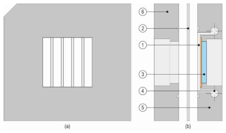
The key element of the experimental stand was a test module containing five parallel minichannels (see the view in Fig. 1a). Each minichannel had the following dimensions: 1 mm depth, 6 mm width, and 43 mm length. A schematic longitudinal cross-section of the test module is shown in Fig. 1b. The module was closed with two aluminium-alloy covers, and the side walls of the minichannels were formed using a Teflon foil. The heated wall was made of a thin Haynes-230 alloy foil (thickness of approximately 0.1 mm) and was electrically powered by resistive (Joule) heating, providing a controlled and spatially uniform heat flux.
The working fluids were low-boiling refrigerants: HFE-649, HFE-7100, and HFE-7200. The fluid flowed horizontally above the lower heated wall of the minichannels. The centrally located minichannel was selected as the representative (model) channel for numerical modelling and data reduction.
Research method
During the experiments, heat transfer and flow resistance (pressure drop) were investigated under controlled operating conditions. The key measured parameters included the working fluid temperature and pressure at the inlet and outlet of the central minichannel, the mass flow rate, and the wall temperature distribution on the outer surface of the heated foil obtained by infrared thermography. Flow patterns in the minichannels were also observed and recorded using a high-speed video camera. Data acquisition and post-processing were carried out with a dedicated measurement system integrated with software for real-time recording, visualisation, and monitoring of the experimental parameters.
Before each measurement series, the working fluid was degassed and the target thermal and pressure conditions were stabilised. Next, the electrical power supplied to the heating foil was increased stepwise, covering the regime from single-phase forced convection to boiling incipience and further boiling development. For each operating point, inlet and outlet pressure and temperature, mass flow rate, and the electrical current and voltage were recorded at 1 s intervals. In parallel, infrared thermography and high-speed imaging were used to capture the wall-temperature field and the associated flow structures.
Experimental data
The calculations used a set of experimental data recorded at one-second intervals over the 360 s duration of the experiment. The dataset included measurements of the fluid temperature and pressure at the inlet and outlet of the minichannel, the temperature distribution on the outer surface of the heating foil, and the mass flow rate.
Tab. 1 The main measured quantities, ranges, devices and errors.
| Measured parameter | Measu-ring range | Measuring device | Measurement error | |
|---|---|---|---|---|
| Working fluid tempera-ture [K] | at the inlet | 284.05÷ 292.65 | Thermocouple Czaki Thermo-Product type K 221 b | ±0.34 K after individual calibration [20] (Nominal tolerance according to IEC 60584-1 [21] for type-K thermocouples in the relevant temperature range) |
| at the outlet | 286.25÷ 312.85 | |||
| Temperature of the heating foil [K] | 293.42÷ 365.75 | Infrared camera A655sc FLIR (resolution 640 × 480) | ± 2 K or ± 2% in the range of 273.15÷ 393.15 K | |
| Gauge pressure of the working fluid [kPa] | at the inlet | -3.31÷ 57.02 | Pressure meter, Endress+Hauser Cerabar S PMP71 | ± 0.05% of reading |
| at the outlet | -3.86÷ 56.53 | |||
| Atmospheric pressure [kPa] | 95÷98 | Pressure meter Wika A-10 | 0.5% of full scale (0 ÷ 2.5 bar) | |
| Mass flow rate [kg/h] | 20, 40, 60 | Coriolis mass flowmeter, Endress+Hauser Proline Promass A 100 | ± 0.10% of reading | |
| Power supply (electrical para-meters) | Current [A] | 40.44÷ 103.90 | MCC 1608G Dataforth 8B40 | 0.024% of reading; max.0.096 A |
| Voltage [V] | 0.96÷ 2.69 | MCC 1608G Dataforth 8B41 | 0.05% of reading; max. 0.03 V | |
The total mass flow rate was measured upstream of the test module and corresponded to the flow through the whole five-channel system. Since the minichannels had identical nominal geometry and equal cross-sectional area and were supplied through common inlet and outlet manifolds, the mass flow rate in the analysed central minichannel was assumed to be one fifth of the measured total mass flow rate. This value was used to calculate the single-channel mass flux and Reynolds number. The flow rate was not measured separately in individual minichannels; therefore, possible residual channel-to-channel maldistribution, especially under two-phase flow conditions, is treated as a source of experimental and modelling uncertainty.
Main measured quantities, together with their corresponding measurement ranges and errors, are summarized in Table 1. The obtained mean relative errors, amounting to a few percent for subcooled boiling conditions, are discussed in detail in [19,20]. The heat flux was calculated based on the measured current and voltage drops across the heating foil and the known geometric dimensions of the heating foil. The raw experimental data, including the outer-surface temperature of the heating foil measured by infrared thermography as a function of time and distance from the minichannel inlet, as well as the inlet fluid temperature and pressure as functions of time, are shown in Figure 2 for a representative experimental series with HFE-7100 at a mass flow rate of ṁ = 40 kg/h.
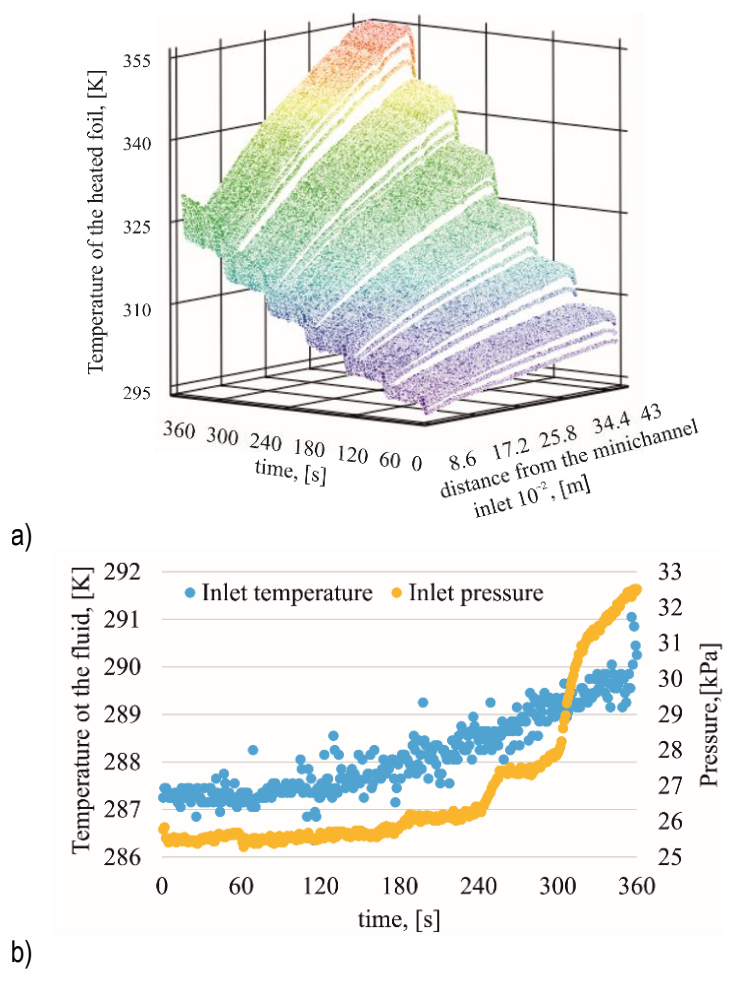
Fig. 2. (a) Temperature of the outer surface of the heating foil, measured by infrared thermography as a function of time and distance from the minichannel inlet, and (b) fluid inlet temperature and pressure as functions of time, for HFE-7100 at a mass flow rate of ṁ = 40 kg/h
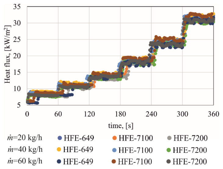
The heat flux calculated from the electrical power input and the heated surface area of the foil, is shown in Figure 3.
Fluctuation analysis of experimental pressure drop
During the experiment, the mass flow rate for each fluid was maintained at an almost constant level of 20, 40, and 60 kg/h, respectively. In each of the nine cases, small fluctuations were observed, characterized by quasi-periodic, wave-like variability. The coefficients of variation of the mass flow rate did not exceed 0.77%. The highest coefficient of variation (0.77%) was recorded at a mass flow rate of 60 kg/h for HFE-649, while the lowest (0.06%) was recorded at a mass flow rate of 40 kg/h for HFE-7100. The flow resistance variation was analyzed under conditions of a stable mass flow rate (coefficients of variation below 1%) using time series analysis methods. The highest pressure drop values were recorded for the highest mass flow rate, with the largest drops obtained for the HFE-7200 fluid, Fig. 4.
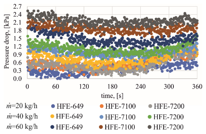
Fig. 4. Pressure drop as a function of time for HFE-649, HFE-7100, and HFE-7200 at mass flow rates of ṁ = 20, 40 and 60 kg/h
The pressure drop was decomposed into trend and cyclical components, i.e. pressure drop fluctuations, enabling the analysis of these fluctuations. An example decomposition for the HFE-7200 refrigerant is shown in Figure 5.
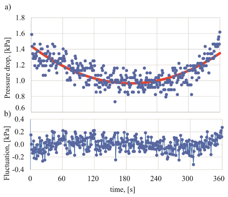
Fig. 5. Decomposition of the pressure drop of the HFE-7200, for mass flow rate ṁ = 40 kg/h, into components: a) pressure drop (blue points) and trend (red line), b) pressure drop fluctuations
Further analysis was conducted exclusively for the pressure drop fluctuations. Their evaluation was performed based on selected statistical parameters: mean, standard deviation, skewness, and excess kurtosis and the analysis of the autoregressive (AR) model. The obtained parameter values indicate that the analyzed data do not deviate significantly from normality with a mean of zero and finite variance. This is confirmed by the calculated mean values of the pressure drop fluctuations, which were on the order of 10-16 kPa low skewness and excess kurtosis values (skewness from −0.21 to 0.21 kPa, kurtosis from −0.45 to 0.12 kPa),as well as the small standard deviation values ranging from 0.092 kPa to 0.119 kPa. The highest standard deviations were observed at the lowest mass flow rate, i.e. 20 kg/h. The analysis of the AR model showed that all roots of the characteristic equation lie outside the unit circle, indicating a stationary nature of the process. In addition, the lack of a dominant frequency suggests that the observed fluctuations of pressure drop do not exhibit characteristics of deterministic oscillations and may be largely associated with stochastic disturbances, including measurement uncertainty.
Flow resistance
The total flow resistance of the fluid flowing in a horizontal minichannel, ((∆p)/(∆L))TP, is the sum of the flow resistance resulting from the friction of the fluid against the walls ((∆p)/(∆L))T and from the change of its momentum ((∆p)/(∆L))A,

To calculate the total flow resistance, the Lockhart-Martinelli separated flow model was adopted, in which the frictional pressure gradient was estimated using the following expression, [22]

where f - the Fanning friction coefficient, L – minichannel length, dh – hydraulic diameter, ρl – density of the working fluid, jl – apparent velocity of the working fluid.
In (2) the two-phase coefficient Φ2 was calculated using the following correlation, [23]

where the subscripts "l" and "v" refer to the liquid and gas phases of the working fluid, respectively.
The Lockhart–Martinelli parameter χ2 was calculated as

The apparent liquid and vapor velocities appearing in the above equations were determined from the relations

The thermodynamic quality, Xth, was determined analogously to that shown in [24]. The Reynolds numbers appearing in equation (4) were calculated using the following relations, respectively

In equations (5) and (6) G is the mass flux, whereas μ is the dynamic viscosity. The subscripts "l" and "v" refer to the liquid and gas phases of the working medium, respectively.
The acceleration pressure drop was determined from the relation, [25]

MATHEMATICAL MODEL AND NUMERICAL METHOD
Heat transfer model
In the mathematical model, the analysis was limited to the length (y) and depth (x) of the central part of the middle minichannel – the heat conduction along the width of the minichannel is neglected. It was assumed that the heat transfer process in the test module is time-dependent, with constant (temperature-independent) thermophysical properties of the heating foil and the flowing fluid. The flow of the refrigerant is laminar (Re < 2300), with a constant mass flow rate and a single velocity component parallel to the flow direction. Under these assumptions, the temperatures of the heating foil TF and the refrigerant Tf satisfy the Fourier-Kirchhoff equation in the form

where: ∇2 = ∂2/(∂x2) + ∂2/(∂y2) denotes the Laplacian operator, q(t) – the heat flux supplied to the heating foil, v(t) – the fluid velocity in a single minichannel, determined on the basis of the mass flow rate obtained from experimental measurements, λ – thermal conductivity, δF – foil thickness, cp – specific heat capacity.
The single-channel velocity was calculated from one fifth of the total measured mass flow rate, as described in Section 2.3. The values of index i and constants a and b in equation (8) for the temperature of two individual domains are given in Table 2.
Tab. 2. Values of index i and constants a, b in equation (8)
| Domain | Index i | Constant a | Constant b |
|---|---|---|---|
| Heating foil | F | 0 | -1 |
| Fluid | f | 1 | 0 |
Equation (8) was supplemented with initial-boundary conditions appropriate for each region. For the foil, it was assumed that: (i) the temperature distribution at its edge is known from thermal imaging camera measurements, (ii) the foil surfaces that are not in contact with the fluid are insulated, and (iii) heat losses to the environment are neglected. For the fluid, the following initial-boundary conditions were assumed: (iv) at the fluid–heating foil interface, temperature continuity is imposed, i.e., the fluid temperature is equal to the heating foil temperature, (v) the fluid temperatures at the inlet and outlet of the minichannel are known from measurements. The adoption of these assumptions leads to the solution of two time-dependent inverse Cauchy-type problems, corresponding to the heating foil and the fluid domains, respectively. Two methods based on Trefftz functions were proposed to solve equation (8): the classical Trefftz method (used to determine the temperature distribution in the heating foil) and a hybrid method combining the Trefftz basis functions with an iterative HPM (used to determine the fluid temperature). Knowledge of the temperature distributions of the heating foil and the fluid at their interface enabled the determination of the Nusselt number based on the Robin boundary condition, i.e.

where: Tf,ave(x,δF,t) reference temperature determined, analogously to [3], as the average temperature of the fluid in the minichannel.
Trefftz functions method and the homotopy perturbation method
The temperature of the heating foil was determined using the classical Trefftz method. The Trefftz functions used are products of functions defined by Rosenbloom and Widder [13] for the one-dimensional Fourier equation. A detailed description of this method and the method for generating time-dependent Trefftz functions can be found in [26,27]. To determine the fluid temperature, a hybrid HPM with Trefftz basis functions was used. Its iterative scheme for time-independent problems can be found in [18,28]. In the HPM, the differential equation (8) for the fluid was written in the form

where Λ and Ν are linear differential operators of the form


In the iterative HPM, the homotopy function h(x,y,t,ξ) is used, which depends, among others, on the parameter ξ where ξ∈⟨0,1⟩ and satisfies the equation

where u0 is an initial solution of equation (10), which satisfies the initial-boundary conditions. Expanding the homotopy h(x,y,t,ξ) into a power series with respect to the parameter ξ as follows

and substituting (14) into (13), and then calculating the limit of the resulting series as ξ→1, gives the solution to equation (10) in the form

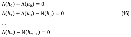
In practice, the fluid temperature Tf is approximated by the sum of a finite series. Substituting (14) into (13) and equating the coefficients at subsequent powers of the parameter ξ, we obtain a system of equations that allows us to iteratively determine the functions h0,h1,h2,…hn, i.e
…
From equations (16) we calculate the subsequent components of the series (15) using the knowledge of the inverse operator Λ-1 given in [27] and the solution of the particular equation (10) in the form

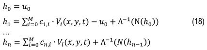
In the first step, it was assumed that the solution to equation (10) is equal to u0 and the following functions h1,h2,…hn are determined iteratively, i.e.
…
where Vi(x,y,t) – Trefftz functions for the linear operator (11), cn,i – unknown coefficients.
Unknown coefficients cn,i of the linear combinations (18) are calculated by minimizing the functional, that describes mean square error of fulfilling initial-boundary conditions.
The temperature fields of the foil and fluid were approximated over the domain (x,y,t)∈[0,L]×[0, δh]×[0, 360 s]. Due to the piecewise (stepped) character of the heat flux (see Fig. 3), the time interval was partitioned into six subintervals, corresponding to successive heating stages. This partitioning yields subdomains of the form [0,L]×[0,δh]×[(k-1)∆t, k∆t] for k =1,…,6 and ∆t = 60s. Within each subdomain, a local approximation of the solution was constructed independently. The foil temperature was expressed as a linear combination of Trefftz functions, while the fluid temperature was represented in the form given by Eq. (15). For each time step k, the initial and boundary conditions were taken from the solution obtained in the previous subinterval (k−1), which ensured temporal continuity of the overall approximation.
The convergence of the hybrid HPM–Trefftz solution follows from two fundamental properties: the completeness of the Trefftz function system and the convergence of the homotopy series. According to the results presented in [26], Trefftz functions are a complete system, which guarantees that the exact solution can be approximated with arbitrary accuracy by Trefftz functions. In [29] the convergence of the HPM series to an exact solution was established under the contraction conditions imposed on the operator. In this case, the proof of convergence follows from the fact that the operator Λ-1(N) is bounded in the considered function space. Consequently, the homotopy perturbation series (15) is convergent under sufficiently small convective perturbations.
The above method for determining the solution of a partial differential equation can be generalized to the case of a nonlinear equation. Then the operator N in formula (12) is a nonlinear operator, and the further calculation procedure is unchanged.
RESULTS
The calculations were performed for experimental data recorded during the first 360 seconds of the experiment for three working fluids, the ranges of which are presented in Table 1. The experimental conditions were identical in terms of the mass flow rate and the heat flux supplied to the heating foil. Differences were noted in the temperature and gauge pressure of the fluid at the minichannel inlet. The highest temperature at the minichannel inlet was recorded for the HFE-7100 while the highest inlet pressure was for the HFE-649. It should be noted that the fluids differ in their physical properties, such as thermal conductivity, heat capacity, density, viscosity, and saturation temperature. These properties influence heat transfer efficiency, boiling development and the time-dependent evolution of the thermal field. These differences directly influence the characteristics of the boiling process and the conditions for its initiation. The thermophysical properties are presented in Table 3.
Tab. 3. Thermophysical properties of the liquids at 25°C; saturation temperature corresponds to the normal boiling point (at 1 atm)
Flow resistance
In determining the frictional flow resistance, the Fanning factor was proposed in the following form

where constants a and b, estimated based on 3240 measurement data, were A = 24.82 and B = 0.0063, respectively. A comparison of the experimental pressure drops with the pressure drops ∆p calculated using formula (1) is shown in Figure 6.
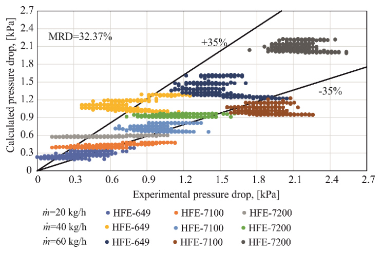
Analysis of the results presented in Figure 6 indicates that nearly 75% of the pressure drop values are within ±35% of the experimental pressure drop values. In three cases, i.e., for HFE-7100 and mass flow rate of 40 kg/h, HFE-649 and mass flow rate of 60 kg/h, and HFE-7200 and mass flow rate of 60 kg/h, more than 95% of the results differ by no more than ±35% from the pressure drops obtained from measurements. The relative differences (RD) in these three cases were also the smallest, below 5%, while the mean relative difference (MRD) for all considered variants was 32.37%. The largest discrepancies were observed for HFE-7100 at a mass flow rate of 60 kg/h. In 65.6% of the cases, the experimental pressure drops were higher than the calculated values.
Figure 7 shows the calculated pressure drop for HFE-649 as a function of time and mass flow rate, while Figure 8 presents the pressure drop values for all the considered cases.
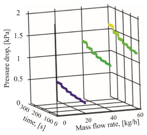
It was observed that the pressure drop increases with increasing mass flow rate and heat flux supplied to the foil. Similar results were obtained for the other fluids.
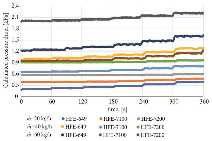
The largest increases in pressure drop over time were observed for HFE-649 and HFE-7100, and these increases were more pronounced at lower mass flow rates. In the case of HFE-7200, no significant changes in pressure drop were observed over time.
Nusselt number calculations
The Nusselt number calculation process consisted of three stages. In the first step, the heating surface temperature was determined using the classic Trefftz method using nine Trefftz functions.
The mean relative difference between the measured and the calculated foil temperatures did not exceed 0.5%, confirming good agreement of the applied approach. Next, the HPM combined with the Trefftz functions was used to determine the two-dimensional temperature distributions of the refrigerants. The HPM expansion was truncated after two terms of the series (15), yielding a first-order approximation [30] that was found sufficient for the considered heat transfer problem in fluid. The final stage was the calculation of the Nusselt number using formula (9).
The Nusselt number as a function of time and distance from the inlet to the minichannel is presented in Figure 9. The results refer to the experiment in which the working fluid was HFE-7200 for mass flow rate ṁ = 60 kg/h.
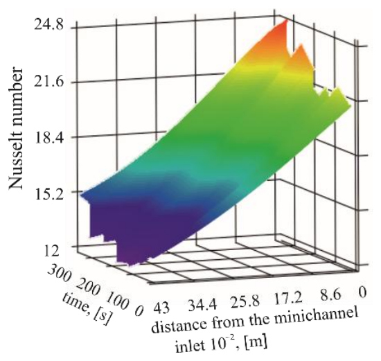
Fig. 9. The Nusselt number as a function of time and distance from the inlet to the minichannel for HFE-7200 and mass flow rate ṁ = 60 kg/h
For HFE-7200 at ṁ = 60 kg/h (Figure 9), the Nusselt number exhibits a clear increase with time, indicating progressive enhancement of heat transfer as the heating programme proceeds. Along the minichannel, Nu is generally higher near the inlet and decreases with increasing distance downstream, which is consistent with an axial development of the thermal/hydrodynamic field. At later times, the surface shows a pronounced high-Nu region (a “peak”), suggesting a transition to a more intensified heat transfer regime within a limited time range rather than a purely linear evolution. Overall, Figure 9 confirms a coupled time-space response: time-driven increasing in heat transfer combined with a persistent axial gradient from inlet to outlet for this operating condition.
The Nusselt number as a function of distance from the minichannel inlet is shown in Figure 10 for selected times (60, 200, and 360 s) for HFE-649, HFE-7100, and HFE-7200 at three mass flow rates.
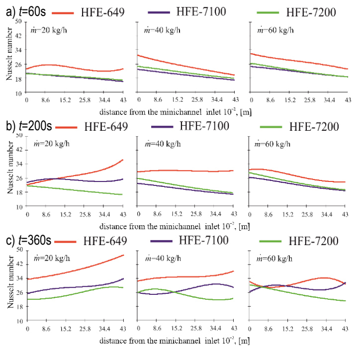
Fig. 10. Nusselt number as a function of distance from the minichannel inlet at selected times: a) t = 60 s, b) t = 200 s, c) t = 360 s, for HFE-649, HFE-7100, and HFE-7200 at three mass flow rates
Analysis of the results presented in Figure 10 indicates that:
At the early stage of the experiment (e.g., Fig. 10a, t = 60 s, lower heat flux), higher mass flow rates yield higher Nusselt numbers for all three fluids. The axial Nu profiles at this stage are predominantly decreasing with distance from the minichannel inlet, consistent with developing-flow (entrance-region) behaviour; however, for HFE-649 at the lowest mass flow rate (ṁ =20 kg/h) the profile remains nearly uniform along the channel length.
At a later stage corresponding to an increased heat flux (Fig. 10b, t = 200 s), HFE-649 exhibits a position-dependent response to mass flow rate: near the minichannel inlet Nu is higher at larger ṁ, whereas for ṁ = 20 kg/h Nu increases markedly along the channel and reaches the highest values in the downstream section. In contrast, for HFE-7100 and HFE-7200 Nu profiles decrease with increasing distance from the minichannel inlet; for these two fluids higher ṁ generally results in higher Nu, with a weaker/non-monotonic response at the lowest mass flow rate for HFE-7100.
At t = 360 s (Fig. 10c), the axial Nu distributions depart from the early-stage, predominantly entrance-region behaviour and become strongly dependent on both the fluid and the mass flow rate. At ṁ = 20 kg/h, Nu increases with distance from the inlet for all three fluids, with the most pronounced rise observed for HFE-649; HFE-7100 and HFE-7200 show a more moderate increase. At ṁ = 40 kg/h, HFE-649 still exhibits a mild axial increase, whereas HFE-7100 and HFE-7200 display clearly non-monotonic profiles with local extrema. At ṁ = 60 kg/h, HFE-7200 shows a predominantly decreasing Nu trend, while HFE-649 and HFE-7100 exhibit pronounced non-monotonic behaviour with curve intersections along the channel length.
These late-stage trends are consistent with differences in boiling development and thermophysical properties (see Table 3). The lower normal boiling point of HFE-649 (322.15 K), favours earlier and stronger boiling enhancement under the same heating programme, which can manifest as increasing Nu downstream (particularly at lower ṁ). In addition, its lower thermal conductivity at 25°C (0.059 W/(m·K)) increases Nu number values for comparable heat transfer coefficient. Conversely, HFE-7200 has the highest normal boiling point (349.15 K) and the highest specific heat (1214 J/(kg·K)), which tend to maintain stronger subcooling and delay boiling enhancement, at higher ṁ this results in more convection-like axial trends, including decreasing Nu. HFE-7100 remains intermediate between HFE-649 and HFE-7200, with mixed (often non-monotonic) axial behaviour indicative of regime transitions along the channel.
Overall, the results show that the Nusselt number depends on time (and thus on the imposed heat flux), but the temporal trend is not universal. In many cases, particularly for HFE-649, Nu increases with time, whereas for HFE-7200 (especially at higher mass flow rates) the increase is weaker and may be replaced by a decrease or non-monotonic behaviour, depending on the axial position.
This diversity is consistent with differences in thermophysical properties and boiling characteristics: the lower normal boiling point of HFE-649 promotes earlier boiling incipience, whereas the higher boiling point of HFE-7200 tends to delay boiling enhancement. In addition, differences in thermal conductivity and specific heat influence both the scaling of the Nusselt number and the evolution of bulk subcooling, contributing to the fluid-specific temporal and axial trends. All three refrigerants have comparable density and dynamic viscosity, suggesting that differences in the hydrodynamic scaling are not the primary driver of the observed inter-fluid trends; rather, the boiling characteristics and thermal properties dominate.
Uncertainty Analysis
To determine the relative errors of the Nusselt number, the standard uncertainty propagation law was applied using the following formula:
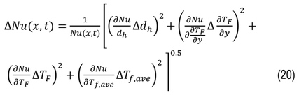
where:

– the uncertainty in the heating foil temperature gradient,

- the uncertainty in the heating foil temperature,

– the uncertainty in the fluid temperature calculated using the HPM combined with the Trefftz method,
∆Tmeas = 2% in the range of 273.15 ÷ 393.15 K – the uncertainty in the heating foil temperature (see Table 1), obtained with infrared camera,
∆t = 0.01s – the uncertainty of the time measurements,
∆Tf = 0.34 K – the uncertainty in fluid-temperature measurements obtained with additionally calibrated K-type thermocouples (see Table 1),
∆dh = 10-4 m – the uncertainty of hydraulic diameter of the minichannel,
∆x = 10-4 m – the uncertainty of the depth of the minichannel.
The analysis of the mean relative errors of the Nusselt number revealed that the uncertainty associated with its determination remained at a comparable level for all investigated working fluids, ranging from approximately 18% to 21%. It was observed that the relative error of the Nusselt number decreased with increasing heat flux supplied to the heating foil, indicating improved accuracy in the determination of heat transfer parameters under higher thermal loads. Among the tested fluids, HFE-7100 exhibited the lowest error values and the narrowest variation with increasing mass flow rate. This behavior may indicate greater stability of the heat transfer process and reduced sensitivity of the calculated results to measurement uncertainties. In contrast, HFE-649 showed the largest increase in relative error with increasing mass flow rate, suggesting a stronger propagation of uncertainties associated with the input parameters used in the calculations. Nevertheless, the differences observed among the investigated fluids were relatively small, indicating that the influence of thermophysical properties, such as density, dynamic viscosity, specific heat capacity, and thermal conductivity, on the overall uncertainty of the Nusselt number determination was limited.
CONCLUSIONS
The paper presents an analysis of calculation results for time-dependent heat transfer during flow boiling of three refrigerants through a set of five parallel rectangular minichannels heated asymmetrically. In the first step of the computational procedure, the Trefftz function method was applied to determine the temperature distribution in the heating foil. Subsequently, the Nusselt number at the interface between the heating foil and the refrigerant was calculated using the HPM. The influence of heat flux and mass flow rate on the Nusselt number values was analyzed. Additionally, the stability of the pressure signal was assessed using statistical time-series analysis methods. Flow resistance was determined based on the separated flow model of Lockhart–Martinelli, in which a new approach for determining the Fanning friction factor was proposed.
Based on the obtained results, the following conclusions were formulated:
In all analyzed cases, the fluid flow in the minichannel was stable (the coefficient of variation of the mass flow rate was less than 1%), and the observed fluctuations in pressure drop had a small amplitude and an approximately normal distribution (the mean value of the resistance oscillated around zero and was characterized by low skewness and kurtosis). The highest values of pressure drop were recorded at the highest mass flow rate, with the largest pressure drops observed for the refrigerant HFE-7200.
The analysis based on the autoregressive (AR) model confirmed the stationary nature of the pressure drop process, and the absence of a dominant frequency indicates that the observed pressure drop fluctuations are mainly stochastic in nature and may be related, among other factors, to measurement uncertainty rather than to deterministic oscillations
For the proposed approach to determining flow resistance, moderate agreement was obtained between the calculated results and the experimental data — in most cases, the differences fell within the assumed deviation range, although some variants exhibited larger discrepancies. In general, the experimental values of pressure drop were higher than the calculated ones. These results indicate the need to improve predictive correlations in order to more accurately estimate flow resistance, particularly under two-phase flow conditions.
The pressure drop increased with increasing mass flow rate and heat flux supplied to the heating foil. The largest time-dependent increases were observed for HFE-649 and HFE-7100, particularly at lower mass flow rate, whereas for HFE-7200 no significant changes over time were found.
The Nusselt number exhibits a clear dependence on time (and thus on the imposed heat-flux programme), but the temporal trend is not universal and depends on the working fluid, mass flow rate, and axial position.
At the early stage (lower heat flux), higher mass flow rates generally yield higher Nu values; the axial profiles are predominantly decreasing with distance from the inlet, consistent with entrance-region behaviour (with HFE-649 at ṁ = 20 kg/h showing an approximately uniform profile).
At later stages (higher heat flux), the influence of ṁ becomes fluid- and position-dependent. In particular, for HFE-649 the inlet Nu is higher at larger ṁ, whereas at ṁ =20 kg/h Nu(x,t) increases strongly downstream and reaches the highest values in the outlet region. For HFE-7100 and HFE-7200 the axial profiles remain predominantly decreasing, with higher ṁ generally giving higher Nu (and a non-monotonic response at the lowest ṁ for HFE-7100).
Among the analyzed refrigerants, the highest Nusselt number values were obtained for HFE-649, with the time-dependent increase being particularly pronounced at lower mass flow rate.
For HFE-7200, the axial Nu(x,t) profiles are predominantly inlet-peaked; the magnitude and time evolution are case-dependent, whereas for HFE-7100 the behaviour is intermediate and often non-monotonic at later times.
The mean relative error of the Nusselt number ranged from approximately 18% to 21% for all investigated working fluids. The results indicate that the uncertainty level was similar regardless of the fluid used, while the relative error decreased with increasing heat flux supplied to the heating foil. Among the tested fluids, HFE-7100 exhibited the lowest and most stable error values.
The observed inter-fluid differences are consistent with the different normal boiling points and thermal properties, which affect boiling enhancement and the scaling Nu; in contrast, the densities and dynamic viscosities are comparable, suggesting that purely hydrodynamic scaling is not the primary driver of the observed trends.
Using the Trefftz function methods (classical and hybrid), time-dependent inverse initial–boundary problems (identification of temperature and heat flux) as well as inverse coefficient problems (identification of the Nusselt number) were solved in two adjoining domains differing in geometry and physical properties. The application of continuous Trefftz functions dependent on three variables (x, y, t) made it possible to avoid domain discretization.
The present study has several limitations. The numerical analysis was restricted to the central minichannel and assumed uniform flow distribution among the parallel channels. In addition, constant thermophysical properties, negligible heat losses, and two-dimensional heat transfer were assumed in the mathematical model. The proposed correlations were evaluated only for the investigated refrigerants, operating conditions, and channel geometry; therefore, further studies are required to extend the applicability of the method to other two-phase flow systems.
NOMENCLATURE
A, B – constant
a, b – constant
c – linear coefficient
AR – autoregressive model
cp – specific heat capacity, J/(kg·K)
dh – hydraulic diameter, m
f – Fanning friction factor
G – mass flux, kg/(s m2)
h – homotopy function
HPM – homotopy perturbation method
j – apparent velocity, m/s
k – number of subdomains
L – minichannel length, m
ṁ – mass flow rate, kg/h
M – number of the Trefftz functions
MRD – mean relative difference
Nu – Nusselt number
p – pressure, Pa
q – heat flux, W/m2
Re – Reynolds number
T – temperature, K
t – time, s
u0 – initial solution
V – Trefftz function
v – velocity, m/s
x, y – coordinates, m
Xth – thermodynamic quality
Greek symbols:
α – heat transfer coefficient, W/(m2·K)
∆ – difference,
∆ – uncertainty,
δ – thickness, m
Λ – differential operator
λ – thermal conductivity, W/(m·K)
μ – dynamic viscosity, kg/(m·s)
Ν – differential operator
ξ – parameter
ρ – density, kg/m3
Φ2 – two-phase friction multiplier
χ2 – Lockhart–Martinelli parameter
∇2 = ∂2/(∂x2) + ∂2/(∂y2) – Laplacian operator