
INTRODUCTION
In recent decades, industries have used robotic systems to automate repetitive or dangerous tasks in industrial applications. In automated processes where the robot moves within its workspace without interacting with the environment, a control system based on position or motion is a viable option. However, as the demands of scientific and technological production processes increase, the tasks assigned to robotic arms are becoming increasingly complex [1]. Motion control has the drawback of requiring a precise model of all the robot’s parameters, which is challenging because complete model information is not always available and often needs to be obtained through regression models [2]. The motion control problem also involves modeling through non-autonomous differential equations, requiring asymptotic stability proofs using strict Lyapunov functions—a non-trivial task [3]. To address this challenge, position control, also known as the regulation problem, simplifies trajectory tracking by using point-to-point control [4]. This approach enables the robot’s end-effector to move to a fixed and constant desired position over time, regardless of its initial joint position. Since the initial position does not affect the system’s stability, the manipulator can trace a series of consecutive points in space (where the previous point serves as the initial condition) that approximate the desired trajectory.
In the regulation problem, the Proportional-Derivative (PD) control law with gravity compensation proposed in [5] ensures global asymptotic stability of the closed-loop system with an appropriate selection of proportional and derivative gains. However, since these gains are constant, abrupt changes in the desired trajectory can increase tracking error, leading some authors to propose variable gains to improve performance. For instance, in [4], researchers propose a solution to the regulation problem by introducing a set of saturated controllers with variable gains. These controllers generate torques within the prescribed limits of the servomotors. The functions for the variable gains allow for smooth self-tuning as the joint position error and velocity approach zero, but it is still necessary to establish parameters for the proportional and derivative gains. In [6], the authors propose a modified neural network algorithm as an adaptive tuning method to optimize the controller gains. The proposal is complex, but robust against uncertainties in system parameters and various trajectories. Unfortunately, it lacks a stability demonstration and requires careful selection of the controller gain limits. The authors of [7] introduce an optimization technique based on an improved Artificial Bee Colony. This technique uses Lyapunov stability functions to determine the optimal gains of a Proportional-Integral-Derivative controller in a 3 degrees-of-freedom manipulator system. The optimized system shows robustness against various perturbation conditions and uncertainty in the payload mass, but the algorithm lacks a stability demonstration, and understanding its operating principle requires considerable effort. Similar observations can be applied to gain tuning using fuzzy algorithms [8]. The authors in [9] propose a regulator with constant proportional gains and variable derivative gains to enhance the robot’s transient response through damping, utilizing position error and velocity. This allows the system to reach a steady state smoothly while meeting the servomotor constraints. Although the results are better than the hyperbolic tangent controller [10], which is known for its effectiveness, tuning still requires designer expertise. In Section 5, we review additional relevant contributions on PD-like controllers with variable gain adaptations [15–23]. The discussion emphasizes the type of controller, the specific structure of the variable gains (e.g. state-dependent, adaptive, fuzzy, or neural-network-based), the stability analysis methods applied (such as Lyapunov theory, singular perturbation theory, or global convergence arguments) and the validation strategies adopted, ranging from numerical simulations to experimental implementations.
In this work, we propose a PD-type position control law for robotic manipulators, where the proportional gains are adjusted as functions of the desired position. These gains are obtained through a Radial Basis Function (RBF) interpolation network trained offline, which reduces online computational demands. The objective is to improve trajectory-tracking performance in terms of accumulated error and energy efficiency when compared to the classical PD regulator [5] and the Tanh regulator [10]. The system’s stability is formally ensured using Lyapunov’s second method. In the remainder of this paper, we denote the proposed approach as the PDN controller. From a theoretical standpoint, PDN does not differ from the classical PD controller of Takegaki–Arimoto [5], since the gains depend solely on the desired position and not on the system states. Consequently, its stability proof is identical to that of the conventional PD law. However, PDN introduces practical advantages: (i) there is no need for re-tuning gains at different desired positions, and (ii) it exhibits enhanced performance in point-to-point trajectory tracking, particularly in terms of robustness, accumulated error, and energy efficiency.
The main contributions of this manuscript can be summarized as follows:
– A methodology for determining the proportional gains of a robotic manipulator controller directly from the desired position, avoiding conventional procedures that depend on designer expertise.
– The use of RBF networks for automatic gain tuning, providing a simpler and more practical implementation compared to alternative methods reported in the literature [6–9].
– Demonstration of improved performance in terms of L2-norm error and energy efficiency in trajectory-tracking tasks with respect to existing approaches.
– Integration of three distinctive features—desired-position dependence, offline RBF training, and Lyapunov-based stability analysis—which together enhance both theoretical guarantees and practical applicability. This combination particularly strengthens point-to-point trajectory tracking and robust regulation without the need for gain re-scheduling, aspects not simultaneously addressed in previous studies.
This work is structured as follows: Section 2 presents the dynamic model of the manipulator robot and the PD regulator. Section 3 discusses the proposed regulator, its stability proof, and the method for training the interpolation networks. Section 4 presents the results of position control and tracking of an owl-shaped trajectory, comparing them with those got from the PD and hyperbolic tangent regulators. A qualitative comparison is presented in Section 5 with state-of-the-art works that employ variable-gain controllers. Section 6 provides the conclusions.
MANIPULATOR DYNAMICS AND PD CONTROL
The dynamic model of a manipulator robot with n degrees of freedom composed of rigid links (see Fig. 1a) can be written as [11]:
where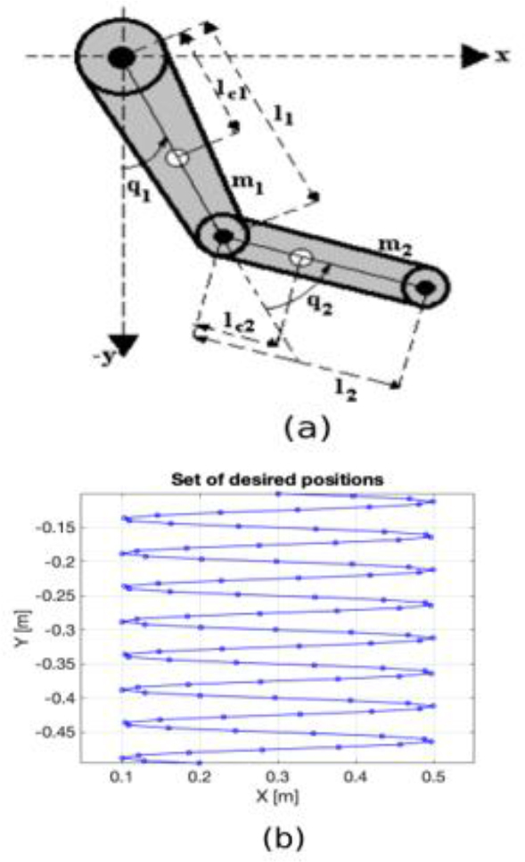
For position control or regulation, the dynamic model can be expressed in closed-loop form as:
where qd = [qd1, qd2, …, qdn]T ∈ ℝn is the vector of desired positions, andPROPOSED PDN CONTROL LAW
The following is a proposed variant of the PD position control that automatically adjusts Kp and Kv based on the desired position, transforming from Cartesian space to joint space through inverse kinematics. The aim is to enhance the controller's performance in trajectory tracking, even when the parameters of the dynamic model (1) are not available. This proposal involves replacing the constant gains Kp and Kv in (5) with diagonal matrices Kp(qd) = diag{kpi(qd)}, Kv(qd) = diag{ρikpi(qd)}, for i = 1, 2, …, n, and ρi ∈ (0,1). The variable gains kpi(qd) and kvi(qd) are scalar functions of qd, the desired position. Each kpi(qd) corresponds to the output of a Radial Basis Function Interpolation Network [12]. Neural networks are used to learn, from data, the nonlinear map from the desired position to effective PD gains, avoiding manual tuning and gain scheduling. The network is trained offline; at runtime only a fast, deterministic mapping is evaluated, reducing commissioning effort and sustaining consistent performance across desired positions. These networks have an input layer, a hidden layer with Gaussian activation functions ϕi, j(qd) for i = 1, 2, …, n and j = 1, 2, …, m, where m is the number of neurons in the hidden layer, and an output layer that sums the activation functions weighted by factors wij [12]. The proposed PD control law is:
where wi, j are the weights of the hidden layer of the interpolation network kpi(qd), Cj ∈ ℝn are the centers of the Gaussian functions, σi are constants that controls the width of the Gaussian functions, and ||·|| denotes the Euclidean distance.. Training Procedure
Next, the following steps detail the procedure for building and training these interpolation networks:
– Design n interpolation networks corresponding to the gains kpi(qd) for each link or degree of freedom.
– Select m desired positions distributed within the manipulator's workspace (see Fig. 1b), which will represent the centers of the Gaussian functions in Cartesian coordinates. Convert them to joint coordinates using the manipulator's Inverse Kinematics. The Inverse Kinematics problem involves calculating the angular displacement vector q based on the orientation and position of the end effector, expressed in reference Cartesian coordinates. The expression for the inverse kinematics of the manipulator shown in Fig. 1a, in the “elbow up” configuration and with reference coordinates (x, y), is [13]:
These samples form the training dataset C={C1, C2,…, Cm}, where Cj ∈ ℝn.
– Perform calibration of the gains kpi and select parameters ρi for the controller in (5) for each position in the set C. The got data will correspond to the training values assigned to the output layer of the n interpolation networks, i.e. {ki1,…, kim}, where kij represents the proportional gain of the i-th joint for the j-th training data.
– Set the value of σi such that the activation of the Gaussian functions in the hidden layer is less than 50%:
with i = 1, 2, …, n, j = 1, 2, …, m, and k = 1, 2, …, m. This value of σi allows the neurons in the hidden layer to specialize in defined regions within the manipulator's workspace. The maximum activation level of these neurons will be reached when the input value is close to their center.– Calculate the weights wij of each network by means of:
– Substitute the values of Cj, and wij in (8) and (9) to get kpi(qd) and kvi(qd) = ρikpi(qd) as functions of the desired position qd.
With this method, n interpolation networks are trained offline.
. Stability proof
The stability proof of (8) using the direct Lyapunov method is similar to that presented in [5] for conventional PD control. Be Kp(qd) = diag{kpi(qd)} and Kv(qd) = diag{ρikpi(qd)}, with kpi(qd) > 0 for all i = 1, 2, …, n. These are not functions of time or system states. Let the Lyapunov candidate function be:
Differentiating with respect to time, we have:
Substituting
15
Simplifying:
which is true if ρikpi(qd) > 0 for all i = 1, 2, …, n and because B > 0. Thus, global stability of the equilibrium pointRESULTS
To validate the PDN control law, simulations were conducted in MATLAB for regulation and trajectory tracking. The trajectory had the shape of an owl within the workspace of the anthropomorphic arm manipulator of Fig. 1a. The parameters of this direct-drive actuator robotic arm are reported in [2, 14], with some of the most important ones shown in Tab. 1.
Tab. 1.
Parameters of the simulated anthropomorphic arm manipulator
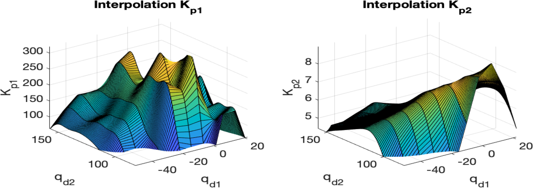
. Interpolation of kp1(qd) and kp2(qd)
The gains kp1(qd) and kp2(qd) of the PDN regulator were adjusted using two RBF interpolation networks (9) and selecting 50 of the 100 desired positions shown in Fig. 1b. The tuning process aimed to optimize the 100 gains to meet the following criteria: less than 1% overshoot, a response time under 2.5 second, τ1<150 Nm, τ2<15 Nm,
. Regulation
Fig. 3 shows the error responses and
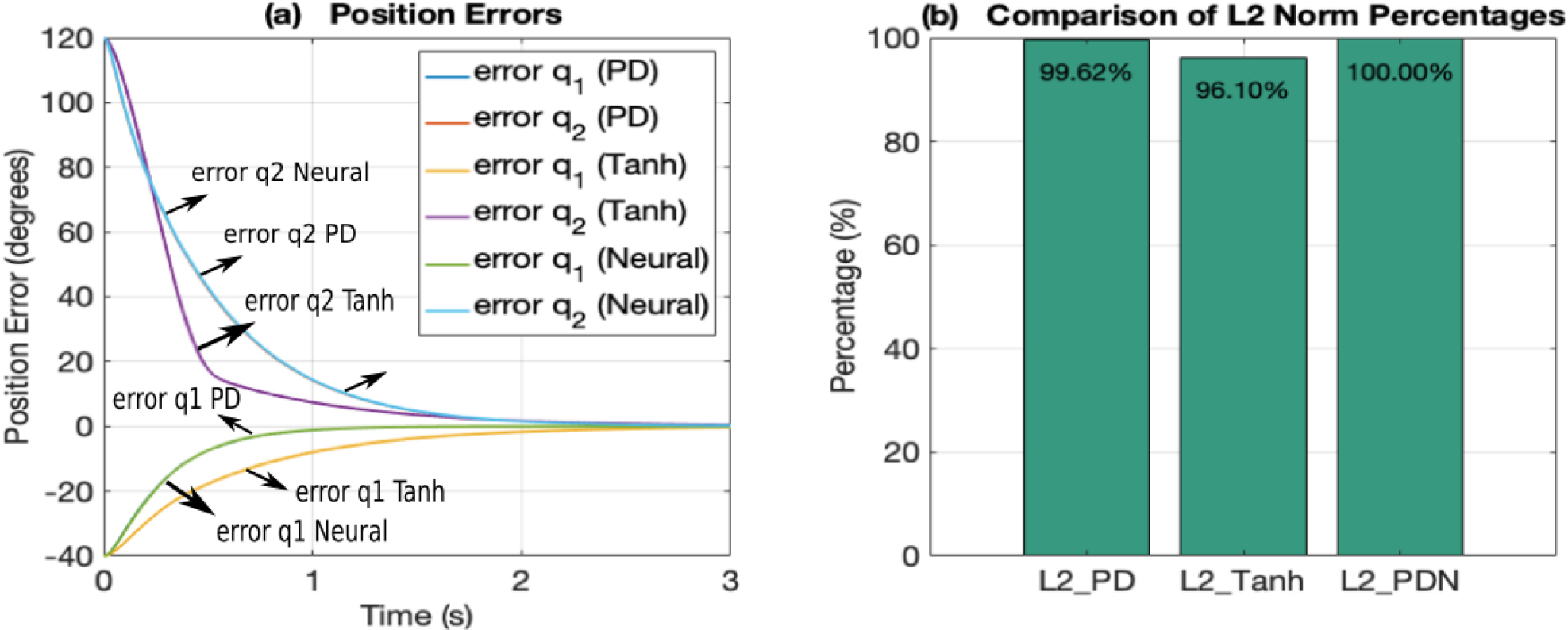
The PD and PDN controllers exhibit very similar position errors (see Fig. 3a), as expected since the PDN regulator was designed based on the PD regulator. In both, the position errors decrease, reaching a steady state in around 2.5 seconds. The Tanh controller shows a less pronounced correction in q1 and a more pronounced correction in q2, but reaching a steady state also around 2.5 seconds. Fig. 3b shows the comparison of the ℒ2 norms of the three controllers.
The PDN controller serves as the 100% reference due to its slightly lower performance. The PD and Tanh controllers have lower ℒ2 norms (less cumulative error), with values of 99.62% and 96.1%. This shows that although all three controllers perform well and similar in terms of position error, the Tanh controller offers a slight advantage by minimizing the ℒ2 norm, suggesting better overall performance in terms of total error energy compared to the other two controllers in the regulation problem. This comparable performance of the three regulators will allow for a meaningful evaluation of their performance in the point-to-point trajectory-tracking problem.
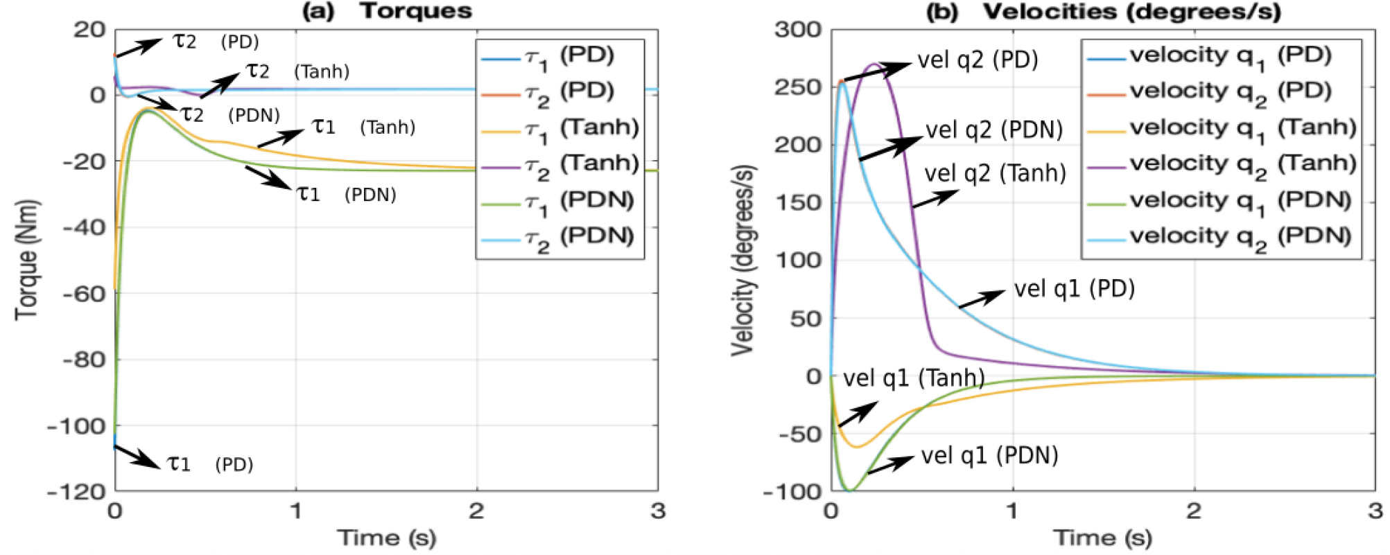
Fig. 4 shows the corresponding torques and angular velocities. As expected, the responses of PD and PDN are practically identical (see Fig. 4a). Both control laws apply similar forces to the manipulator, resulting in equivalent performance. In both cases, torque τ1 shows a sharp negative peak at the start (-107.46 Nm and -102.48 Nm, respectively) before stabilizing near to τ1 = –22.9 Nm, indicating a significant initial effort to correct the position, but still within actuator limit of 150 Nm. Torque τ2 exhibits a smoother behavior, with an initial peak (12.69 Nm in the PD and 11.51 Nm in the PDN, still within actuator limit of 15 Nm) that stabilizes to τ2 = 1.79 Nm. The Tanh regulator generates lower torques than the PD and PDN controllers (τ1 initial of -58.74 Nm and τ2 initial of 5.75 Nm). Additionally, the torque τ1 in Tanh stabilizes more slowly to τ1 = –22.9 Nm, suggesting a behavior with bounded actions. As with the other controllers, torque τ2 is smoother than τ1 and stabilizes to τ2 = 1.79 Nm. The angular velocities in Fig. 4b show that the PD and PDN controllers exhibit almost identical behavior, as expected. In both cases, the velocities of q1 and q2 reach their maximum values and then decreases. The Tanh controller results in a more damped response, especially for q1, showing that its bounded actions result in smoother transitions. In all scenarios, the angular velocities remain within the maximum limits.
To evaluate controller robustness under parametric uncertainty—for example, payload-driven changes in link-2 mass and center of mass—we ran a 200-trial Monte Carlo with truncated Gaussian perturbations (±15%) applied to all the Tab. 1 coefficients with the desired position (qd1, qd2) = (–40°, 120°).
The Fig. 5 overlays the nominal error response (black) with shaded ±1 standard deviation bands, and Fig. 6 shows boxplots of robustness metrics obtained by Kruskal-Wallis and bootstrap analyses. Qualitatively, PD exhibits the tightest dispersion and quickest convergence in the q1 error; PDN shows similar transients but a wider spread, consistent with PD gains being hand-tuned for this set-point while PDN gains are produced by a neural estimator not tailored to the operating point. For q2, all controllers decay rapidly, but Tanh is visibly poorer and with larger spread.
Fig. 5.
Monte Carlo robustness of PD, Tanh, and PDN controllers under parametric uncertainty and (qd1, qd2) = (–40°, 120°)
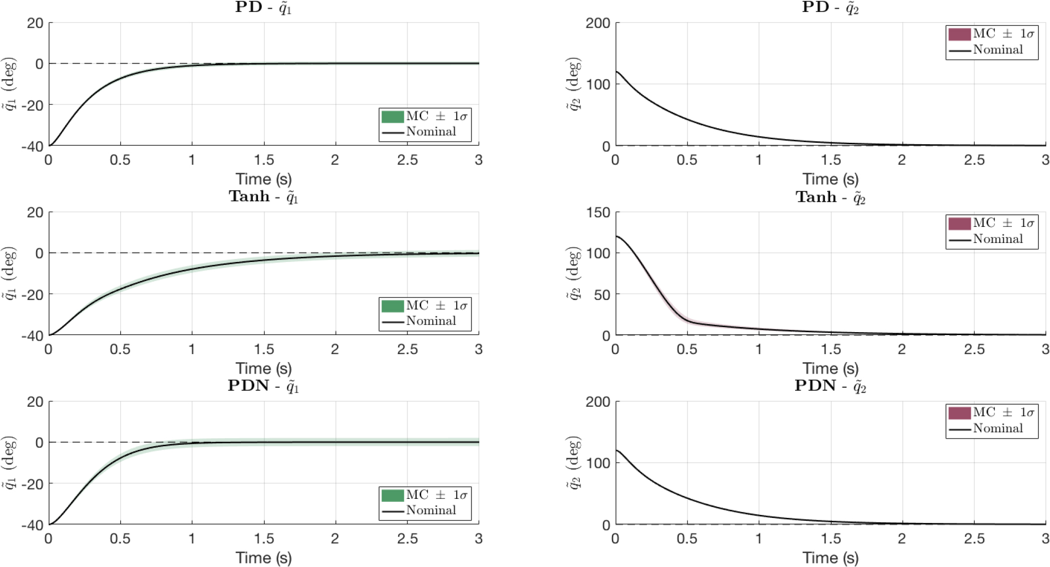
Fig. 6
Boxplots of robustness metrics (Ts, e(ts), ISE, and ℒ2 – i. e., ∥e∥2 –) for PD, Tanh, and PDN controllers with (qd1, qd2) = (–40°, 120°), ±15% parametric uncertainty, and 200 Monte Carlo trials
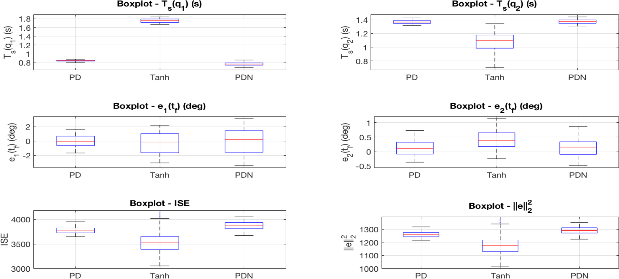
Because the Monte Carlo metrics were non-Gaussian (normality rejected by a Lilliefors/Kolmogorov–Smirnov test), we used Kruskal–Wallis and complemented it with bootstrap 95% confidence intervals for the medians. The analysis confirms strong between-controller differences for settling time Ts(q1) (significance p<0.05): PDN attains the smallest median Ts(q1) = 0.773 s with confidence interval [0.768, 0.779], a 56.1% improvement over the worst case (Tanh).
For Ts(q2) (p<0.05), Tanh is fastest with median 1.117 s [1.068, 1.150], 19.0% better than the worst (PDN). Steady-state error at final time, e1(ts), shows no significant differences (p=0.068), whereas e2(ts) does (p<0.05); PD yields the lowest median e2(ts) = 0.185 deg [0.068, 0.260], a 32.8% reduction relative to Tanh. Integrated error measures also differ markedly (p<0.05): Tanh achieves the smallest ISE (median 3573) and the lowest time-normalized error ℒ2 (median 1191), about 8.2% better than PDN. Overall, PDN is fastest in joint-1, Tanh is fastest in joint-2 and most favorable in energy-like errors, and PD minimizes steady-state error for joint-2.
To analyze the effect of PDN self-tuning—while keeping the gains of the other controllers fixed at the values used for the (qd1, qd2) = (–40°, 120°) operating point—we pooled the Monte Carlo data across the three set-points (-40°, 120°), (0°, 90°), and (–20°, 140°) and applied a Kruskal-Wallis test; the results are as follows. For settling time Ts(q1), groups differ (p<0.05); PDN attains the lowest median 0.7725 s, improving by 56.2% over the worst (Tanh). For Ts(q2), groups differ (p<0.05); Tanh is best with median 1.100 s, a 19.1% improvement over the worst (PDN). For steady-state error e1(ts), differences are not significant (p ≥ 0.05). For e2(ts), groups differ (p<0.05); PDN is best with median 0.1163 deg, a 55.9% reduction relative to the worst (Tanh). For the integral metrics, ISE andℒ2, groups differ (p<0.05); Tanh achieves the lowest medians (ISE = 3529, ℒ2 = 1176), each 9.3% better than the worst (PDN). Overall, across the three operating points, PDN is fastest in joint-1 transients, Tanh is fastest in joint-2 and most favorable for energy-type errors, and PD does not dominate but remains competitive in steady-state bias for joint-2.
Therefore, we observe that, for regulation tasks, the PDN controller is competitive with PD and Tanh, even with parametric uncertainty, but its main advantage is that it does not require manual tuning of the proportional and derivative gains.
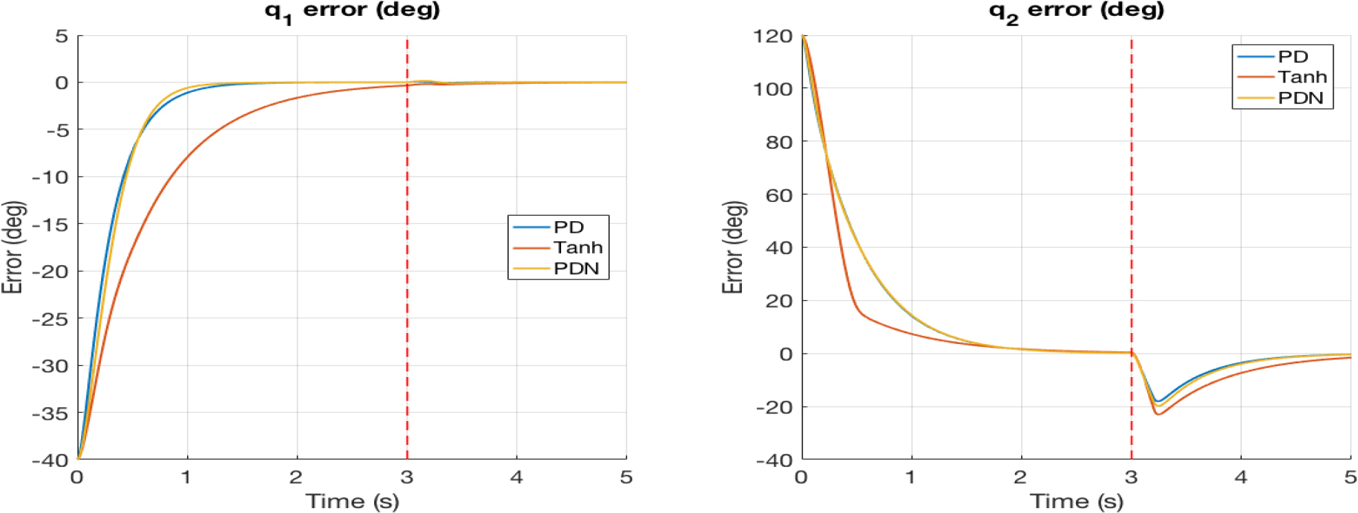
In Fig. 7, an external disturbance was applied at joint 2: a 6 Nm torque starting at t = 3 s and lasting 0.15 s (red dashed line). In q1 the impact is minor and short-lived due to limited coupling; all controllers keep the error close to zero with only a small blip. In q2 the disturbance causes a pronounced negative excursion (about –20 to -25 degrees), which reveals clear differences in disturbance rejection: PD shows the smallest excursion and the fastest recovery, PDN is a close second with a slightly deeper dip and slower return, and Tanh performs worst with the largest dip and the longest tail. This ranking aligns with controller structure: PD and PDN retain linear behavior to counter a torque pulse, whereas the Tanh controller soft-limits the proportional and derivative actions, reducing corrective effort.
. Point-to-point trajectory tracking
Fig. 8a shows the ideal trajectory that the robot should follow, represented in the shape of an owl interpolated from 200 points and completed in 25 seconds. The PDN controller permits the robot to track this trajectory with a sampling period of 2.5 ms, corresponding to 10,000 samples, as illustrated in Fig. 8b. The Tanh and PD controllers yield similar results. Fig. 8c and Fig. 8d show the joint velocities for the Tanh and PDN controllers. In both cases, the velocities of joints q1 and q2 remain near the saturation limits. However, the Tanh controller achieves higher velocity values, although it stabilizes more quickly, which affects its energy consumption. The energy consumption is calculated as:
Fig. 8.
Point-to-point "Owl" trajectory tracking. (a) Ideal trajectory. (b) Trajectory with the PDN controller. (c) Actuator speed with the Tanh controller. (d) Actuator speed with the PDN controller. (e) Comparison of ℒ2 norms. (f) Comparison of energy consumption.
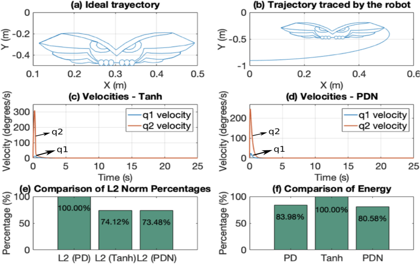
Fig. 8e and Fig. 8f compare the performance regarding the ℒ2 norm and energy consumption. Unlike the regulation control case, in trajectory tracking, the PDN controller shows the best performance in terms of accumulated position error, with the lowest ℒ2 norm (73.48%), followed by the Tanh controller (74.12%) and then the PD (taken as the 100% reference). This shows that the PDN controller better minimizes the accumulated error. Regarding energy consumption, the PDN controller also stands out with the best performance (80.58%), followed by the PD (83.98%), and the Tanh (100%, taken as the reference). Besides reducing the error, the PDN controller is also more energy-efficient.
DISCUSSION
In agreement with Tab. 2, the proposed controller differs from previous variable-gain PD approaches in several key aspects. While many studies introduce variable gains as functions of state variables (e.g., position, velocity, or error) [15–23], our approach uniquely defines the proportional gain as a function of the desired position. This structural distinction has important implications:
– Offline Training and Practical Implementation: Unlike methods that rely on adaptive or iterative online updates [15, 17, 21], the proposed controller employs an RBF interpolation network trained offline. This design reduces online computational burden, making the method more practical for real-time applications without sacrificing performance.
– Formal Stability Guarantees: Several previous works either omit stability analysis [16, 18, 19, 23] or provide only limited claims (e.g., “global convergence” without detailed proofs) [19]. In contrast, our control law is rigorously validated through Lyapunov theory, ensuring global asymptotic stability under both trajectory tracking and regulation tasks.
– Point-to-Point Tracking and Regulation without Re-tuning: Whereas prior approaches often require parameter re-adjustment depending on trajectory complexity or regulation scenarios, our method demonstrates strong performance in point-to-point tracking while also showing that regulation tasks can be achieved without re-tuning the gains.
Tab. 2.
Comparative table of studies on PD controllers with variable gains
| Study | Controller Type | Variable Gain Structure | Stability Analysis Method | Validation Approach |
|---|---|---|---|---|
| [4] | PD-like with variable gains | Variable; state-, position-, and velocity-dependent; smooth functions (e.g. cos2 (tanh (error+velocity))) | Lyapunov theory; global asymptotic stability; gravity compensation required | Simulation; two-DOF direct-drive robot; joint regulation; L2 norm |
| [15] | PD iterative neural-network learning (PDISN) | Likely variable/adaptive; neural network and iterative learning | Extended Lyapunov theories; stability type not specified | Simulation; manipulator characteristics not specified; scenario not specified |
| [16] | Proportional-derivative (PD) | Variable; tuned by self-organizing fuzzy algorithm | Not analyzed (no details) | Simulation; manipulator characteristics not specified; tracking control; position error metric |
| [17] | Self-tuning PD | Bounded, time-varying; neurofuzzy recurrent scheme | Lyapunov theory; semi-global exponential stability | Simulation; manipulator characteristics not specified; trajectory tracking |
| [18] | Nonlinear PID with fuzzy self-tuned PD gains | Variable, position-dependent; fuzzy logic | Not mentioned; global asymptotic stability; no gravity compensation | Experiments; type not specified; scenario and metrics not specified |
| [19] | Adaptive PD | Adaptive to gravity parameters | Not mentioned; global convergence | Simulation; three-DOF manipulator; point-to-point and tracking |
| [20] | PD-type robust | Variable, error-varying; parameterized by perturbing parameter | Singular perturbation theory; stability type not explicit | Physical experiment; planar two-DOF direct-drive robot; trajectory tracking |
| [21] | Adaptive iterative learning control (ILC)-PD | Variable; iterative learning, two iterative variables | Lyapunov theory; asymptotic convergence | Simulation; two-DOF manipulator; trajectory tracking |
| [22] | PD-type | Variable, state-dependent | Not mentioned; global asymptotic stability claimed | Physical experiment; two-DOF directdrive arm; scenario not specified |
| [23] | Linear and nonlinear PD-type | Nonlinear functions of system states | Not mentioned; global asymptotic stability claimed | Simulation; single-link and two-DOF robots; trajectory tracking |
| This work | PD-like with variable gains | Variable; desired position dependent proportional gains with RBF interpolation networks trained offline | Lyapunov theory; global asymptotic stability; gravity compensation required | Simulation; two-DOF direct-drive robot; joint regulation; L2 norm, point-to-point tracking; regulation performance evaluated with parametric uncertainties and external perturbations |
This makes the controller particularly suitable for manipulators executing sequences of set-points, as the stability and efficiency remain robust across tasks.
– Robustness to Uncertainties and Perturbations: While some works include robustness studies under limited assumptions [20], the proposed control law explicitly evaluates performance under parametric uncertainties and external perturbations, confirming its reliability in realistic operating conditions.
CONCLUSIONS
Compared to the existing literature, the proposed controller combines three distinctive contributions-desired-position dependence, offline RBF training, and formal Lyapunov stability-which together enhance both theoretical guarantees and practical applicability. Its strength lies particularly in point-to-point trajectory tracking, where the error is reduced in a more energy-efficient form regarding PD and Tanh controllers. It also presents robust regulation without gain re-scheduling, aspects that are not simultaneously addressed by previous studies.