
INTRODUCTION
Robotic manipulators are widely recognized as essential components in modern automation, space exploration, and industrial systems due to their ability to perform precise, reliable, and repetitive tasks in complex environments. Continuous advancements have focused on improving structural design, control strategies, and adaptability to enhance performance under uncertain and dynamic conditions. For instance, a 6-DOF manipulator developed for space applications integrates lightweight structures, high-precision actuators, and advanced inverse kinematics with teleoperation capabilities, enabling efficient handling of objects with varying geometries [1]. To improve control performance under uncertainties, several advanced control strategies have been proposed. Robust adaptive fuzzy sliding mode controllers combine fuzzy logic with adaptive mechanisms to enhance trajectory tracking and disturbance rejection [2]. Similarly, adaptive robust control methods incorporating neural network-based parameter estimation have been developed for cooperative manipulators, ensuring accurate trajectory and force tracking even in the presence of base coordinate uncertainties [3]. In addition, dynamic control approaches incorporating obstacle avoidance and space operator algebra, along with multi-loop PID structures, have been shown to reduce torque fluctuations, improve motion smoothness, and enhance energy efficiency [4]. Beyond control strategies, significant research has also focused on kinematic modelling, dynamic analysis, and trajectory planning of robotic manipulators. Studies on inverse and forward kinematics have addressed joint constraints, redundancy, and workspace optimization to improve manipulator performance [6], [8], [12]. Dynamic modelling approaches have been developed to analyse forces, torques, and system stability using simulation environments such as MATLAB/Simulink and multibody formulations [15], [17]. In addition, trajectory planning and path optimization techniques, including RRT-based methods and intelligent optimization strategies, have been widely investigated for efficient motion generation in complex environments [32], [33]. Despite these advancements, a review of existing work reveals several limitations. Advanced control techniques often require accurate system modelling and complex parameter tuning, making them less suitable for simplified simulation environments. Furthermore, many path planning studies are evaluated independently and lack integration with kinematic and dynamic models of the manipulator. Simulation-based approaches frequently do not provide interactive user control or fail to combine kinematics, dynamics, and path planning within a unified framework. Moreover, most trajectory tracking analyses rely on closed-loop control strategies, limiting their applicability in open-loop simulation studies.to address these challenges, this work proposes a MATLAB/Simulink-based integrated framework for a 4-DOF robotic manipulator. A CAD model is imported into Simscape Multibody to achieve realistic physical modelling, while both forward and inverse kinematics are implemented to establish the relationship between joint space and Cartesian space. Path planning is performed using A*, Dijkstra, and RRT algorithms under identical conditions, followed by interpolation and spline-based smoothing to generate feasible and continuous trajectories. Additionally, a MATLAB App Designer based graphical user interface (GUI) is developed to enable inter active control and visualization. Dynamic analysis is conducted to evaluate joint forces, torques, velocities, and motion smoothness within an open-loop simulation environment. The main contribution of this work is the development of a unified and computationally efficient simulation framework that integrates path planning, kinematics, and dynamics for a 4-DOF manipulator. A comparative evaluation of A*, Dijkstra, and RRT is performed using metrics such as path length, computation time, and explored nodes, along with trajectory smoothing for improved motion feasibility. The inclusion of an interactive GUI enhances usability and visualization, while dynamic analysis provides insights into actuator performance and system efficiency. Unlike many existing approaches, the proposed framework avoids complex control dependencies and hardware requirements, making it cost-effective and suitable for academic research and educational applications.
LITERATURE SURVEY
N. Sreekanth et al. developed a 6-DOF lightweight and reconfigurable robotic manipulator for space exploration using tele-motion control and a customized inverse kinematics approach. Its adaptive end effector efficiently handles both symmetric and asymmetric objects [1].Xiuxing Yin et al. designed a robust adaptive fuzzy sliding mode controller for uncertain serial manipulators, employing fuzzy logic to approximate uncertainties and adaptive laws for real-time tuning, achieving superior tracking and robustness [2].Anbang Zhai et al. proposed a neural network-based adaptive robust controller for cooperative manipulators operating under uncertain base coordinates, ensuring accurate trajectory and force convergence [3].Huihui Hong et al. presented a dynamic obstacle-avoidance control using space operator algebra and a three-loop PID to minimize torque fluctuation and motor energy loss while enhancing smoothness [4].Neeraj Mishra et al. analyzed a human-arm robotic arm under different loading conditions using FEA in Ansys, emphasizing material optimization to improve durability and cost-effectiveness [5]. Rutong Dou et al. developed a 7-DOF humanoid arm with analytical-reverse order kinematic solutions and a global arm angle optimization algorithm validated through ROS simulations [6].Guoliang Zhong et al. introduced a continuum manipulator of NiTi alloy with a co-radial configuration and a displacement-compensation-based inverse kinematics method verified through experiments [7].Yanlin Chen et al. proposed a 7-DOF redundant manipulator optimized via Linearly Decreasing Weight PSO to minimize motion time, validated through geometric modeling and experiments [8].Cheng-Hsuan Yang et al. presented a collision-avoidance strategy for modular construction robots using a sampling-based planner, achieving over 80% success in avoiding collisions [9].Dileep Rao et al. designed a 4-DOF surgical robotic manipulator with a state observer-based controller that enhances precision and minimizes torque requirements compared to PID [10].Swet Chandan et al. analyzed a 7-DOF manipulator using D-H parameters and optimized joint angles via PSO and Firefly algorithms to improve trajectory accuracy [11].Shubh Shrey et al. performed forward and inverse kinematic modeling of a 5-DOF Lynx6 arm in MATLAB, showcasing workspace visualization and potential for surgical applications [12].A. Zahedi et al. presented kinematic and dynamic modeling of hybrid agricultural robots using recursive algorithms, enhancing crop harvesting precision and efficiency [13].Yi Liu et al. developed a 7-DOF redundant robot for spacecraft assembly optimized via GA, B-spline, and NSGA-2 for improved accuracy and load capacity [14].Alexandru Bârsan et al. modeled the KUKA KR210-2 robot using Simulink-Simscape and validated torque data experimentally through a forming process [15].Kaushik Patel et al. investigated dynamic effects of actuator inertia on an RSSR-SS parallel manipulator using Newton–Euler formulation and MATLAB-SolidWorks simulation [16].Claudio Urrea et al. introduced automated dynamic equation derivation software in MATLAB using Lagrange–Euler formulation with MPC integration for motion optimization [17].Shabnom Mustary et al. modeled a flexible UR5 manipulator using Lagrangian mechanics and fuzzy logic, showing stiffness as the most critical factor for stability [18].Mohammad Sheikh Sofla et al. developed a model-based sliding-surface controller for continuum manipulators using fluidic muscles, ensuring stability under sudden loads [19].Thanh-Trung Do et al. formulated dynamics for flexible-joint manipulators using the Lagrangian approach, validated experimentally for modal accuracy [20].Cheng Zhang et al. built a dynamic model of the MG400 robotic arm in Simscape with variable-gain iterative learning control to enhance tracking accuracy [21]. Lauri Pyrhönen et al. proposed a system identification and force estimation method using a semirecursive multibody model and Kalman filtering on the TX40 manipulator [22].Mihai Dupac et al. proposed trajectory generation for redundant manipulators using spherical coordinates and Hermite interpolation to reduce joint velocity and energy [23].Weiguang Yu et al. developed a time-optimal multi-point trajectory planner using sine jerk and adaptive algorithms for smooth, efficient motion [24].Ozge Ekrem et al. applied PSO-based fifth-order polynomial trajectory planning in MATLAB for vibration-free 6-DOF robotic arm motion [25].Zhou Jiang et al. implemented a fractional-order PID controller optimized by FBPA-PSO to improve trajectory tracking precision and minimize overshoot [26].Hanyi Huang et al. integrated AFC with ANFIS, iterative learning, and reinforcement learning to enhance trajectory tracking in SCARA robots [27].Muhammad I. Azeez et al. optimized a PID controller using the Golden Jackal Optimization algorithm for a 3-DOF manipulator, ensuring Lyapunov stability and robustness [28].Zied Ben Hazem et al. developed a dynamic model of the Mitsubishi RV-2AJ 5-DOF arm, where an ANFIS controller outperformed PID in complex trajectories [29].Claudio Urrea et al. compared MPC, PD-PI fuzzy, and computed torque control methods for a 3-DOF manipulator, achieving high tracking accuracy [30].Guobin Si et al. refined A* path planning with fuzzy PID for mobile robots, improving efficiency and adaptive obstacle avoidance [31]. Junhui Yi et al. proposed a modified version of the RRT* algorithm that incorporates goal biasing and Bézier curve fitting, resulting in improved convergence speed and smoother trajectory generation for robotic manipulators.[32]. Meilin Kang et al. proposed an improved bidirectional RRT algorithm incorporating dynamic expansion strategies, which reduces path length and computational time for orchard robot navigation. [33]. Safa Jameel Al-Kamil et al. used motion-capture-based path planning for industrial robots, improving control accuracy and collision avoidance [34]. Ruipeng Liu et al. proposed an improved RRT* (Rapidly-exploring Random Tree Star) for motion planning of free-floating space robots capturing tumbling objects, achieving enhanced trajectory smoothness and reduced energy consumption [35].
METHODOLOGY
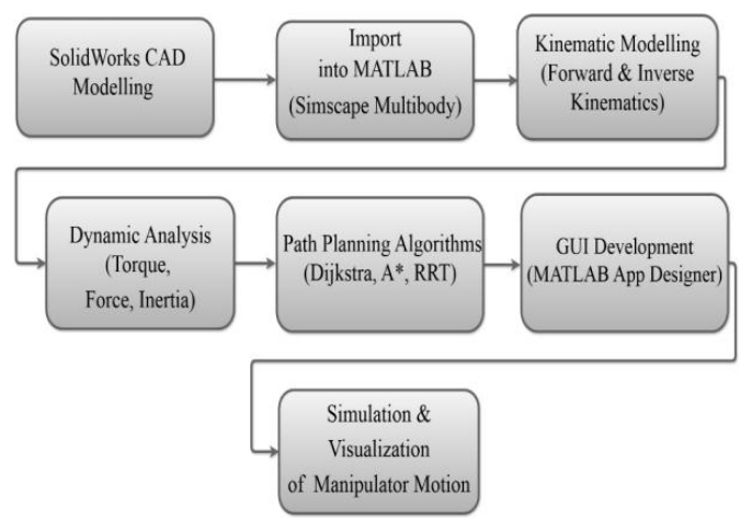
The block diagram of the proposed system, shown in Fig. 1, illustrates the complete workflow adopted for the design, modelling, analysis, and control of a 4-DOF robotic manipulator. The process begins with SolidWorks CAD Modelling, where the 3D structure of the manipulator is created, including links, joints, and the base. This model is then imported into MATLAB via Simscape Multibody, which converts the CAD design into a physics-based simulation environment, preserving geometric and mechanical constraints. Once imported, kinematic modelling is carried out, where forward kinematics is used to determine the end-effector position from given joint angles, and inverse kinematics is applied to calculate joint angles for a desired end-effector position. This ensures accurate motion control and forms the mathematical basis of the system. Following this, dynamic analysis is performed using built-in sensors in Simscape to capture torque, force, and inertia values, allowing evaluation of the manipulator’s physical performance under operational conditions. The next stage involves path planning algorithms, where classical methods such as Dijkstra, A*, and RRT are implemented to generate optimized trajectories for manipulator motion. To enhance user interaction, a Graphical User Interface (GUI) is developed in MATLAB App Designer, enabling real-time visualization and manual control of the manipulator. Finally, the entire framework is validated through simulation and visualization of manipulator motion using MATLAB Simulink and Simscape Mechanics Explorer. This stage ensures that the integrated system performs as expected, bridging the gap between theoretical design and practical implementation. Overall, the block diagram highlights the systematic approach of combining CAD modelling, mathematical analysis, intelligent algorithms, and user interactivity to create a comprehensive virtual testbed for robotic manipulator design and control.
The flowchart shown in Fig. 2 illustrates the complete workflow for modelling and simulation of the 4-DoF robotic manipulator using SolidWorks and MATLAB Simulink. The process begins with the creation of a 3D CAD model in SolidWorks, where each link and joint is designed to accurately represent the kinematic structure of a four-degree-of-freedom revolute manipulator. After finalizing the mechanical model, it is exported as a STEP file using Simscape Multibody Link, which enables conversion of CAD geometry into a Simulink-compatible format. This STEP file is then processed in MATLAB to generate an XML file containing the structural hierarchy and physical parameters of the system.
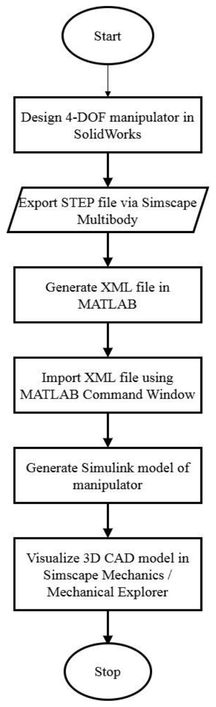
The XML file is subsequently imported into Simulink using the smimport function in MATLAB Simscape Multibody. Here, smimport is a MATLAB function that converts CAD-based XML descriptions into an equivalent Simscape Multibody model, including links, joints, coordinate frames, and constraints. The generated model is then simulated and visualized in Simscape Mechanics Explorer, enabling real-time 3D observation of the manipulator motion. This simulation framework serves as the foundation for integrating control strategies, applying joint torques, and evaluating kinematic and dynamic performance in subsequent stages.
The flowchart shown in Fig. 3 represents the workflow adopted for the design and implementation of the proposed 4-DOF robotic manipulator system with integrated path planning and control. The process begins with the creation of a user-friendly Graphical User Interface (GUI) in MATLAB App Designer, which serves as the central platform for interacting with the manipulator model.
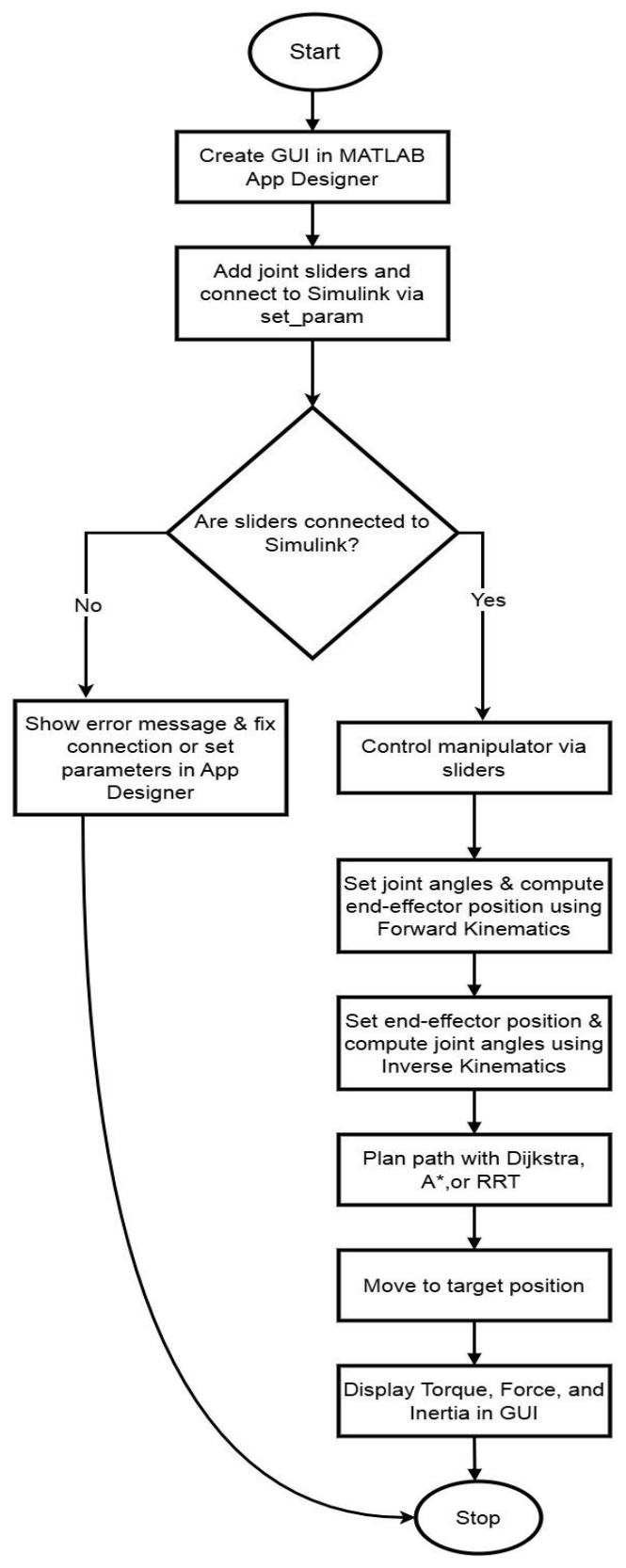
Joint sliders are then added to the GUI and connected to the Simulink environment using the set_param function, enabling real-time parameter updates and control. A conditional check is performed to verify the proper connection between the sliders and the Simulink model. If the connection fails, the system provides an error message, allowing the user to fix the link or reset the parameters in App Designer. Once the connection is established, the manipulator can be controlled interactively through the sliders. Forward kinematics calculations are carried out to determine the end-effector’s position based on the given joint angles, while inverse kinematics computations are employed to obtain the required joint angles for a specified end-effector target position. For motion planning, classical and intelligent algorithms such as Dijkstra, A*, and RRT are integrated to generate trajectories, ensuring efficient navigation in dynamic environments. The manipulator then moves to the computed target position based on the selected trajectory. During this process, dynamic parameters including torque, force, and inertia are sensed through the revolute joint blocks in Simscape and displayed in the GUI for real-time feedback. This workflow ensures smooth integration of kinematic modelling, path planning, and dynamic analysis into a unified simulation environment, thereby bridging theoretical concepts with practical visualization and enhancing the system’s applicability for research and industrial purposes.
Frame assignment
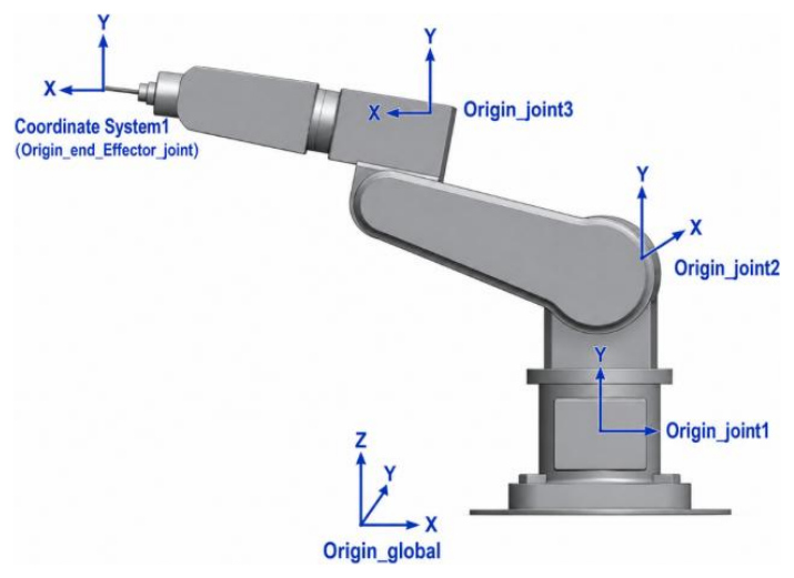
The Fig. 4 coordinate frames for the 4-DOF robotic manipulator are assigned following the standard Denavit–Hartenberg (DH) convention to ensure systematic kinematic modelling. The base frame (Frame 0) is defined at the global origin (origin global), with the Z0-axis oriented vertically upward, representing the axis of the base, and the X0-axis aligned in the forward direction. Frame 1 is attached at the first joint (origin_joint1), where the Z1-axis coincides with the axis of base rotation (vertical axis), and the X1-axis is directed along the first link.
Frame 2 is assigned at the shoulder joint (origin_joint2), with the Z2-axis aligned with the shoulder rotation axis and the X2-axis oriented along the upper arm link. Similarly, Frame 3 is defined at the elbow joint (origin_joint3), where the Z3-axis corresponds to the elbow rotation axis and the X3-axis follows the forearm direction. Finally, Frame 4 is attached at the end-effector (origin_end_effector_joint), with the Z4-axis representing the tool axis and the X4-axis aligned along the end-effector direction. This frame assignment ensures that each joint rotation is represented about its respective Z-axis, enabling consistent formulation of forward and inverse kinematics for the manipulator.
Denavit–Hartenberg (DH) parameters
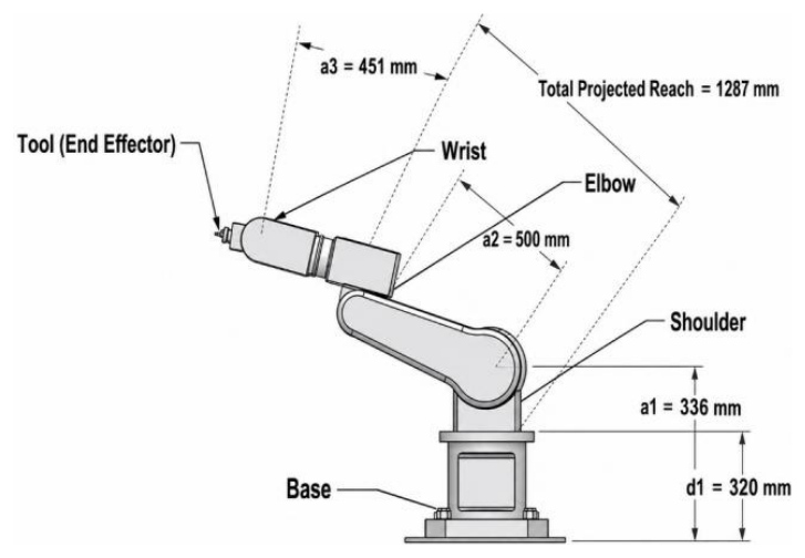
Fig. 5. Dimensional layout of a robotic manipulator highlighting link lengths, joints, and total reach
The above Fig. 5 To represent the manipulator systematically, the standard Denavit–Hartenberg (DH) convention is used. Each link of the manipulator is described in terms of four parameters: link length, link twist, link offset, and joint angle. These parameters are organized in a DH table, which forms the basis for deriving the transformation matrices between consecutive links.
Tab. 1. Denavit–Hartenberg parameters for 4-DoF manipulator
| Joint (i) | Link Length | Link Twist α | Link Offset | Joint Angle θ |
|---|---|---|---|---|
| 1 | a1 | 0 | d1 | θ1 |
| 2 | a2 | 0 | 0 | θ2 |
| 3 | a3 | 0 | 0 | θ3 |
| 4 | a4 | 0 | 0 | θ4 |
The Tab. 1 kinematic configuration of the manipulator is described using standard Denavit–Hartenberg (DH) parameters, which provide a systematic way to represent the spatial relationship between consecutive links. The link length ai represents the distance between two successive joint axes measured along the common normal (typically aligned with the Xi-axis). The link twist αi defines the angle between two consecutive Z-axes, representing the relative orientation between adjacent links. The link offset di denotes the distance measured along the Z-axis from one joint to the next, which remains constant for revolute joints and varies only in prismatic joints. Finally, the joint angle θi represents the rotational displacement about the Z-axis and serves as the primary variable for revolute joints. Together, these parameters enable a complete mathematical description of the manipulator’s geometry and are essential for deriving forward and inverse kinematics.
Forward and inverse kinematics
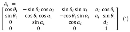
The forward kinematics of the 4-DOF robotic manipulator is formulated using the standard Denavit–Hartenberg (DH) convention. Each joint transformation is represented by the homogeneous transformation matrix given in (1):
The overall transformation matrix of the end-effector is obtained as shown in (2):

This transformation provides the position and orientation of the end-effector.
The inverse kinematics problem determines the joint angles required to reach a desired end-effector position defined in (3):

The base joint angle is computed as given in (4):

The radial distance and vertical offset are defined in (5) and (6):


Using the cosine law, the elbow joint angle is obtained from (7) and (8):


The shoulder joint angle is calculated as shown in (9):

Finally, the wrist joint angle is given in (10):

Joint limits
Joint limits define the allowable range of motion of each joint and are implemented in this work as bounded constraints within the MATLAB-based graphical user interface and Simulink model. In the proposed 4-DoF manipulator, all revolute joints are assigned a range of –180° to 180°, representing software-defined (soft) limits that enable full rotational freedom during simulation. This choice is motivated by the need to explore the complete kinematic behaviour of the manipulator and to simplify user interaction in the GUI environment. Within the Simscape Multibody framework, these limits ensure that the joint inputs remain within a predefined range during simulation, thereby avoiding undefined or numerically unstable configurations. However, it is important to note that these limits correspond to an idealized model and do not necessarily reflect physical actuator constraints or mechanical stops. In practical robotic systems, joint limits are typically narrower and asymmetric, which would further restrict the feasible joint space and, consequently, the reachable workspace. Nevertheless, in the present work, the use of symmetric ±180° limits provides a comprehensive evaluation of kinematic performance, inverse kinematics solutions, and path planning behaviour under unconstrained rotational conditions, while still maintaining bounded and controllable simulation inputs.
Workspace (Jacobian/singularity)
In this work, the workspace of the 4-DoF robotic manipulator is defined as the set of all end-effector positions obtained by varying the joint angles within the limits implemented in the MATLAB GUI and Simulink model. Since all joints are allowed to rotate within –180° to 180°, the manipulator is able to explore its maximum kinematic capability in simulation. The workspace is not derived analytically but is visualized directly in Mechanical Explorer, where the motion of the manipulator is observed in a three-dimensional environment.Based on the link dimensions used in the model (approximately a2=500 mm,a3=451 mm, and base offset d1=320 mm, the end-effector can reach positions within a rotationally symmetric volume around the base axis. The outer boundary of the workspace is defined by the maximum extension of the arm (sum of link lengths), while an inner region near the base remains unreachable due to geometric constraints of the links. As a result, the workspace appears as a three-dimensional dome-shaped or spherical-like volume with a hollow inner region, which is consistent with articulated robotic arms.Since the manipulator is simulated in Simscape Multibody, the workspace representation inherently reflects realistic kinematic behaviour, including link constraints and joint motion. The use of full rotational limits (–180° to 180°) ensures that the displayed workspace corresponds to an extended theoretical workspace, allowing comprehensive visualization of all reachable positions within the simulation environment. This approach provides an intuitive and practical understanding of the manipulator’s reachability without requiring separate analytical derivation, as the workspace is directly observed through the simulated motion of the robot in Mechanical Explorer.
Path planning algorithms
Dijkstra's algorithm is a graph-based path planning method that finds the shortest path between a start node and a goal node by iteratively expanding the node with the lowest cumulative cost. In this study, the edge cost is computed using the Euclidean distance between adjacent nodes.The edge cost between two adjacent nodes is computed using the Euclidean distance is given by

A* is a heuristic search algorithm that combines the advantages of Dijkstra's shortest path search with heuristic guidance toward the target location. The total evaluation cost is defined in (12)

where g(n) represents the accumulated cost from the start node to node n, and h(n) denotes the estimated cost from node n to the goal. In this study, the heuristic function is calculated using Euclidean distance. By incorporating heuristic information, A* reduces the number of explored nodes while maintaining near-optimal path quality. Consequently, the algorithm provides a suitable balance between computational efficiency and trajectory optimality.
Rapidly-Exploring Random Tree (RRT) is a sampling-based path planning algorithm designed for efficient exploration of high-dimensional search spaces. The algorithm incrementally constructs a tree structure by randomly generating samples within the workspace and connecting them to the nearest existing node. The process continues until a feasible path connecting the start and goal positions is established. Unlike Dijkstra and A*, RRT prioritizes exploration and path feasibility rather than strict path optimality. As a result, the generated trajectories may be longer and less smooth, but the algorithm is highly effective in complex environments where exhaustive graph search becomes computationally expensive.
Tab. 2. Path planning parameters
The path planning parameters used for comparison of all the three algorithms is presented in Tab. 2. Planning was performed in Cartesian space, where the end-effector moved from the specified start position to the target position within the manipulator workspace. For A* and Dijkstra algorithms, Euclidean distance was used as the path cost metric, while A* additionally employed the Euclidean heuristic function to guide the search toward the goal. The RRT algorithm utilized uniform random sampling for workspace exploration. After path generation, the resulting waypoints were transformed into joint-space trajectories using inverse kinematics and subsequently smoothed using cubic spline interpolation to ensure continuous and physically feasible manipulator motion.
Trajectory Planning Framework
In the proposed system, path planning is performed in Cartesian (task) space, where the end-effector position is defined by the coordinates (x,y,z). The user specifies the target position through a graphical user interface (GUI), and the input is constrained within predefined workspace limits to ensure feasibility. Accordingly, both the start and goal positions are represented as points in Cartesian space, and the path planning algorithms generate a sequence of intermediate waypoints connecting them. Although planning is carried out in Cartesian space, the manipulator operates in joint space defined by the joint vector given in (13)

Therefore, a transformation from Cartesian space to joint space is required for execution, which is achieved using inverse kinematics, ensuring that each Cartesian waypoint corresponds to a valid joint configuration.
The cost function depends on the selected path planning algorithm. For graph-based algorithms such as Dijkstra and A*, the cost is defined based on the Euclidean distance between nodes, representing the path length. In the case of A*, the total cost function is given in (14)

where g(n) represents the accumulated cost from the start node to node n, and h(n) denotes the heuristic estimate of the remaining distance to the goal. In contrast, the Rapidly-exploring Random Tree (RRT) algorithm focuses on feasible path generation through random exploration rather than strict optimality, and therefore does not explicitly minimize a global cost function.
To ensure safe and physically feasible operation, several constraints are incorporated during trajectory generation. The workspace constraints restrict the target position within the reachable region of the manipulator, defined in (15) as

Based on the link dimensions and validated through Simscape Multibody simulation. Additionally, joint limits are imposed such that

as shown in (16), ensuring that all computed joint angles remain within allowable actuator bounds. Furthermore, smoothness constraints are applied to avoid abrupt motion, maintaining continuity in position, velocity, and acceleration.
Following path generation, each Cartesian waypoint is transformed into joint angles using inverse kinematics, represented in (17) as:

This results in a discrete joint-space trajectory defined in (18):

Only valid inverse kinematics solutions are accepted; if a feasible solution does not exist for any waypoint, the trajectory is rejected. The discrete trajectory is refined to ensure smooth execution. Interpolation is used to maintain a uniform number of trajectory points, followed by cubic spline smoothing defined in (19) as:

which ensures continuous motion. Additionally, a Savitzky–Golay filter may be applied to reduce noise and smooth higher-order derivatives. Finally, the smoothed trajectory is executed sequentially through integration with the simulation environment, where joint values are updated via the GUI, transmitted to Simulink using the set_param function, and visualized in Simscape Multibody Mechanical Explorer. A fixed delay is introduced between successive trajectory points, providing implicit time parameterization and ensuring gradual and continuous motion of the manipulator.
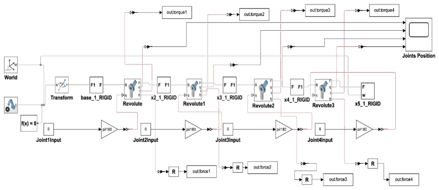
The modelling shown in Fig. 6 represents the 4-DOF robotic manipulator was modelled and simulated in MATLAB Simulink using the Simscape Multibody environment, which enables physics-based analysis of multibody systems. The model consists of a fixed world reference frame connected to the manipulator base through a transform block, while the manipulator itself comprises four rigid links connected via revolute joints. Each revolute joint is actuated using angular inputs, which are converted from degrees to radians before being applied, thereby ensuring precise joint-level motion control. Forward kinematics was implemented to determine the position and orientation of the end-effector for given joint angle inputs, enabling evaluation of workspace and trajectory tracking. Inverse kinematics was employed to compute the required joint variables corresponding to a specified end-effector target, which facilitates task-based positioning and motion planning. To extend the framework beyond basic kinematic modelling, classical path planning algorithms such as Dijkstra, A*, and Rapidly-exploring Random Tree (RRT) were integrated into the simulation for trajectory generation. These algorithms were employed to produce optimized joint-space and task-space paths that ensure smooth end-effector motion between start and goal configurations. In addition to kinematic modelling, the dynamic behaviour of the manipulator was analysed by incorporating inertial properties of the links and extracting joint torques and reaction forces during simulation. The torque outputs quantify the actuation effort required under different motion conditions, whereas the force outputs represent link interaction forces, thereby providing insight into structural loading and dynamic performance. This integrated kinematic, dynamic, and trajectory planning framework not only enables comprehensive analysis of the manipulator’s behaviour but also establishes a foundation for the development of advanced control strategies and real-time human–machine interaction through MATLAB App Designer.
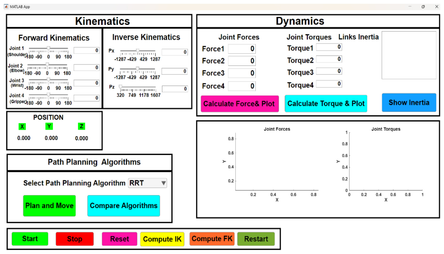
The flowchart shown in Fig. 7 represents a graphical user interface (GUI) was developed in MATLAB App Designer to facilitate the control, analysis, and visualization of the 4 DOF robotic manipulator. The interface integrates kinematic, dynamic, and trajectory planning functionalities within a unified platform. In the kinematics module, forward kinematics is realized through joint angle sliders that allow intuitive manipulation of the four revolute joints, while the corresponding end-effector position in Cartesian space is updated in real time. The inverse kinematics functionality enables users to specify a target end-effector position (Px, Py, Pz), from which the required joint configurations are automatically computed. The dynamics module provides quantitative evaluation of manipulator behaviour by displaying joint forces, joint torques, and link inertial properties, with options to calculate and visualize torque and force responses under different conditions. The path planning module incorporates classical algorithms such as Dijkstra, A*, and Rapidly-exploring Random Tree (RRT), allowing users to select an algorithm, generate trajectories, and compare results across methods. Additional control features, including Start, Stop, Reset, Restart, and dedicated functions for computing FK and IK, enhance interactivity and streamline testing. This GUI thus serves as a comprehensive tool that integrates modelling, control, and trajectory generation, enabling both intuitive operation and systematic performance assessment of the robotic manipulator.
RESULTS AND DISCUSSION
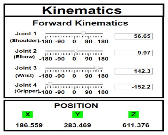
MATLAB App interface developed for the practical implementation of forward kinematics in a 4-DOF robotic manipulator. Is shown in Fig. 8.
The interface enables interactive variation of joint angles (shoulder, elbow, wrist, and gripper) through sliders, with real-time computation of the end-effector position. For the configuration Joint 1 = 56.65°, Joint 2 = 9.97°, Joint3= 142.3°, and Joint4 = –152.2°, the end-effector position was determined as X=186.559 mm, Y=283.469 mm, Z=611.376 The results confirm the accuracy of the forward kinematics model and highlight the effectiveness of the GUI-based control for real-time visualization of manipulator configurations.
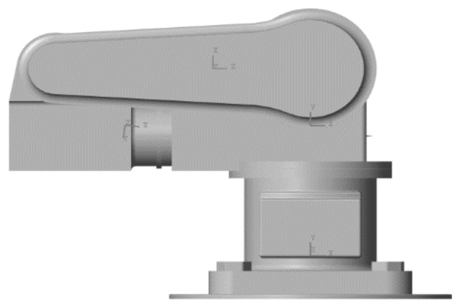
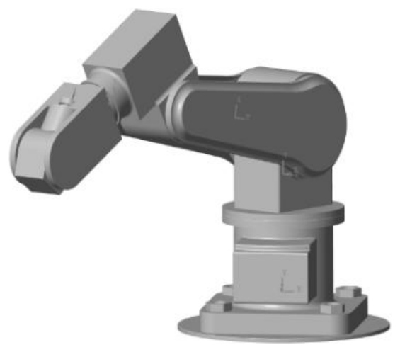
The Fig. 9 shows the manipulator at its initial position in the 3D Mechanical Explorer, representing the default joint configuration before performing forward kinematic computations. The Fig. 10 illustrates the manipulator in the configuration obtained from the forward kinematics model, where the computed joint angles are applied to reach the desired Cartesian position. This visualization validates the correctness of the kinematic formulation, as the simulated pose in the 3D environment matches the theoretical results calculated in the MATLAB App. The consistency between the analytical computations and the simulated model confirms the accuracy of the forward kinematics approach. Furthermore, this implementation establishes a solid foundation for advanced tasks such as trajectory planning, motion control, and inverse kinematics, ensuring that the manipulator can be effectively controlled within its defined workspace.
The Fig.11 illustrates the implementation of inverse kinematics for the 4-DOF manipulator. The interface allows the desired end-effector position (Px,Py,Pz) to be specified via sliders or numerical input, after which the inverse kinematics algorithm computes the corresponding joint angles (shoulder, elbow, wrist, and gripper).
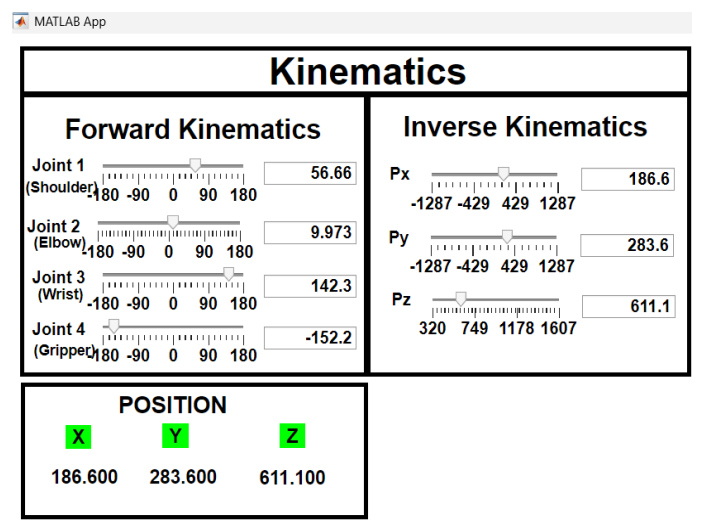
For the target position Px=186.6 mm, Py=283.6 mm, Pz=611.1 the computed joint values were Joint 1 = 56.65°, Joint 2 = 9.97°, Joint 3 = 142.3°, and Joint 4 = –152.2°, which match the forward kinematics results, thereby validating the accuracy of the inverse kinematics model.
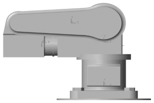
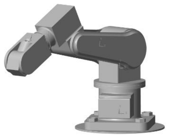
The Fig.12 shows the manipulator at its initial position in the 3D Mechanical Explorer, representing the default home configuration of all joints before executing kinematic computations. From this reference pose, joint displacements are applied to achieve the desired motion. The Fig. 13 illustrates the manipulator moving within the 3D Mechanical Explorer environment, visually confirming the correctness of the computed joint values. This synchronized motion validates that the manipulator accurately reaches the specified Cartesian coordinates in simulation, consistent with both forward and inverse kinematics results. Furthermore, the implementation underscores the role of inverse kinematics in robotic control, as it enables the automatic determination of joint configurations for trajectory tracking and task execution within the workspace.
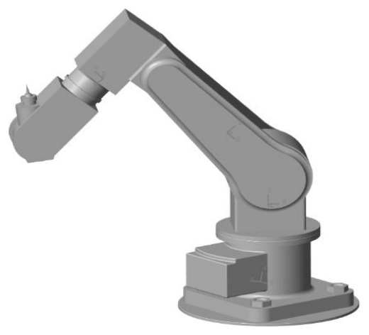
The Fig.14 presents the 3D model of the 4-DOF robotic manipulator developed in MATLAB Simscape Multibody. The model provides a realistic representation of the manipulator’s structure and motion based on the computed joint configurations, serving as a visual validation of the kinematic results. This simulation facilitates understanding of how variations in joint parameters affect the manipulator’s posture and workspace.
The Fig.15 illustrates the MATLAB App interface developed for dynamics analysis of the 4-DOF manipulator. The interface allows specification of the desired end-effector position (Px,Py,Pz), after which the inverse kinematics algorithm computes the required joint angles.
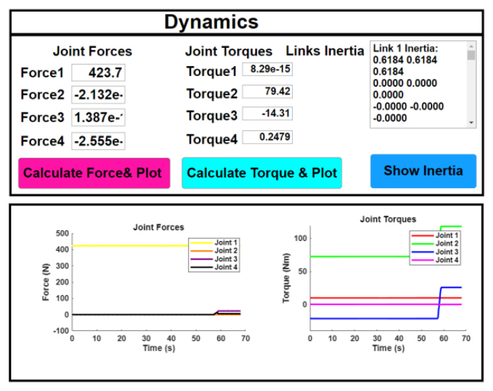
Once the target configuration is achieved, the corresponding joint forces, torques, and inertia properties are calculated. These results are presented numerically and visualized through time-based plots of joint forces (N) and torques (Nm), while the inertia tab provides link-specific inertial parameters, offering insights into the manipulator’s dynamic behavior.
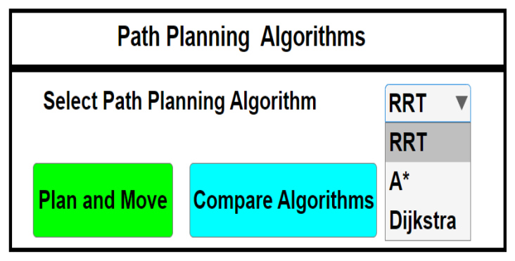
The Fig. 16 shows the MATLAB App interface for robotic path planning, where the user selects an algorithm (RRT, A, or Dijkstra) from the dropdown menu and presses the “Plan and Move” button. This triggers the path planning process, where the chosen algorithm computes a feasible trajectory from the current position to the specified goal.
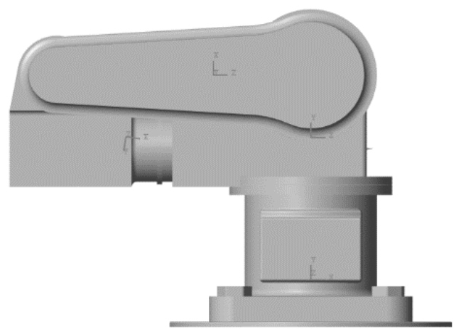
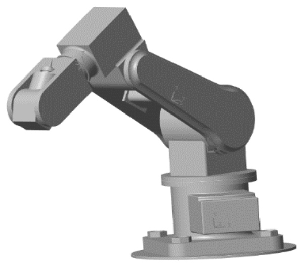
The Fig. 17 shows the manipulator at its initial position in the 3D Mechanical Explorer, representing the starting configuration before executing any path planning algorithms. The planned Cartesian path is then translated into joint space using inverse kinematics, enabling the robotic arm to perform the motion. The Fig. 18 presents the 3D model of the manipulator after executing the planned trajectory. In all cases, the robot successfully follows the generated path, with the end-effector reaching the defined target position while the joints remain within their kinematic limits. This validates the effectiveness of the implemented path planning algorithms in achieving accurate and reliable robotic motion.
The validation methodology employed in this study is limited to simulation-based analysis. The effectiveness of the implemented path planning strategies was evaluated by comparing Dijkstra, A, and RRT algorithms under identical start and goal conditions. Performance metrics included path characteristics, computational efficiency, and trajectory smoothness. The resulting Cartesian trajectories were converted into joint-space trajectories through inverse kinematics and validated within the Simscape Multibody environment.
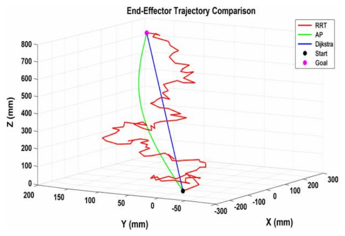
Fig. 19. Comparison of end-effector trajectories using RRT, A*, and Dijkstra path planning algorithms
Fig. 19 presents a three-dimensional comparison of end-effector trajectories generated using RRT, A*, and Dijkstra's algorithm. The trajectories are plotted in Cartesian space along the X, Y, and Z axes (in mm). The motion starts from the initial position [0,0,0] and reaches the goal position [259,178.8,728].The RRT trajectory (red) exhibits a highly irregular and non-smooth path due to its random sampling nature, which makes it suitable for complex and obstacle-rich environments but less optimal in terms of path quality. In contrast, the A* trajectory (green) demonstrates a smoother and more efficient path by incorporating heuristic guidance toward the goal. The Dijkstra trajectory (blue) represents the shortest path in terms of cost; however, it lacks smoothness due to the absence of heuristic optimization.Overall, A* provides a balanced performance in terms of path optimality, smoothness, and computational efficiency, making it well-suited for the considered manipulator application.
Fig. 20 illustrates the end-effector trajectories generated using RRT, A*, and Dijkstra's algorithm for a different goal position. The motion is represented in Cartesian space, where the starting position is [0,0,0] and the goal position [350,178.8,728]. The black marker denotes the start point, while the magenta marker indicates the target position.The RRT trajectory (red) follows a non-smooth and irregular path due to its exploratory nature. The A* trajectory (green) provides a smoother and more directed path by leveraging heuristic-based search. The Dijkstra trajectory (blue) appears as a straight-line path representing the minimum cost solution, but it does not explicitly consider smoothness.This comparison highlights that A* achieves a suitable trade-off between path optimality and smoothness, while Dijkstra ensures minimum distance and RRT emphasizes feasibility in complex search spaces.
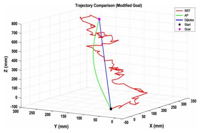
Fig. 20. End-effector trajectory comparison for a different target position using RRT, A*, and Dijkstra algorithms under changed input conditions
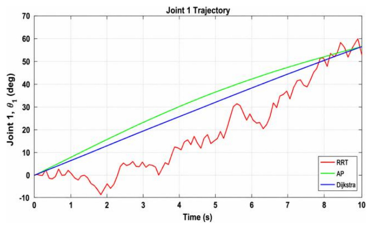
Fig. 21 illustrates the angular trajectory of Joint 1 over time for three different path planning algorithms: RRT, A*, and Dijkstra. The RRT trajectory (red) exhibits noticeable fluctuations and irregularities due to its stochastic and exploratory nature, resulting in a less smooth motion profile. In contrast, the A* trajectory (green) shows a smoother and more progressive increase, indicating a more optimized and guided path toward the target configuration. The Dijkstra trajectory (blue) follows a straight linear interpolation, representing a uniform and steady change in joint angle without any consideration for dynamic smoothness. Overall, A* provides a balance between smoothness and efficiency, while RRT introduces variability, and Dijkstra maintains simplicity but lacks adaptability to dynamic conditions.
Fig. 22 illustrates angular trajectory of Joint 2 over time for RRT, A*, and Dijkstra path planning algorithms. The RRT trajectory (red) shows significant fluctuations with abrupt changes, reflecting its random exploration behavior and lack of smoothness in motion. The A* trajectory (green) demonstrates a smooth, curved profile with a gradual rise followed by slight stabilization, indicating an optimized and controlled path toward the target configuration. Meanwhile, the Dijkstra trajectory (blue) follows a straight and steady linear progression, representing uniform motion without adaptation to dynamic variations. Overall, A* achieves a smoother and more efficient trajectory, RRT introduces variability and instability, and Dijkstra provides a simple but less flexible solution.
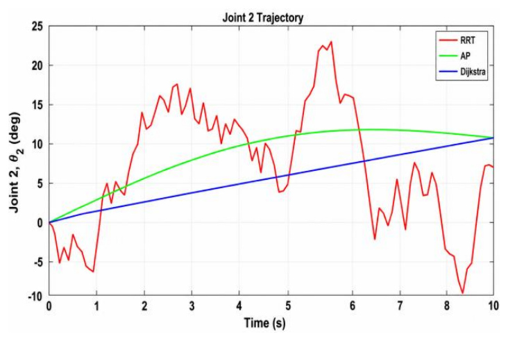
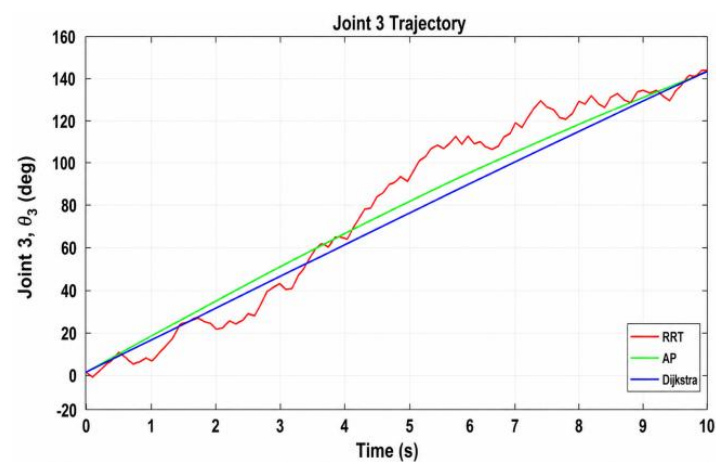
Fig. 23 illustrates the angular trajectory of Joint 3 over time for the RRT, A*, and Dijkstra path planning algorithms. The RRT trajectory exhibits noticeable fluctuations and slight deviations from the desired path due to its random and exploratory nature, resulting in a less smooth motion profile. In contrast, the A* trajectory follows a smooth and steadily increasing curve, indicating an efficient and optimized path toward the target configuration. The Dijkstra trajectory shows a linear and uniform progression, representing a simple interpolation without considering dynamic smoothness. Overall, the A* algorithm demonstrates superior smoothness and efficiency, while RRT introduces variability, and Dijkstra provides a consistent but less adaptive trajectory.
Fig. 24 presents the angular trajectory of Joint 4 over time for the RRT, A*, and Dijkstra path planning algorithms. The RRT trajectory shows noticeable fluctuations and irregular deviations throughout the motion due to its stochastic sampling nature, resulting in a less smooth and less predictable profile. In contrast, the A* trajectory follows a smooth and consistent decreasing trend, indicating an optimized and controlled path toward the desired final position. The Dijkstra trajectory exhibits a straight linear decrease, representing uniform interpolation without accounting for smoothness or dynamic constraints. Overall, A* provides a well-balanced and smooth trajectory, while RRT introduces variability, and Dijkstra offers simplicity but limited adaptability.
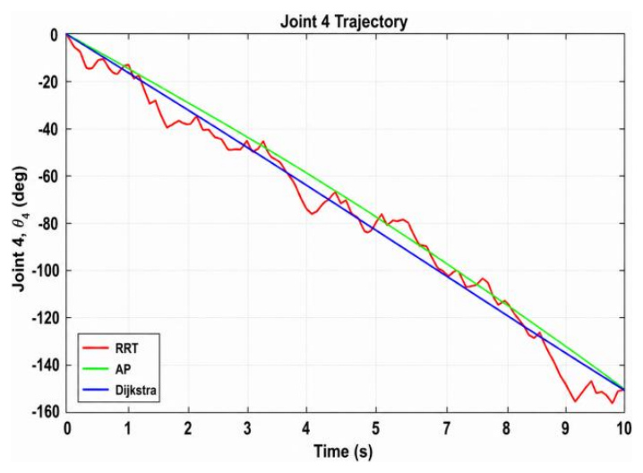
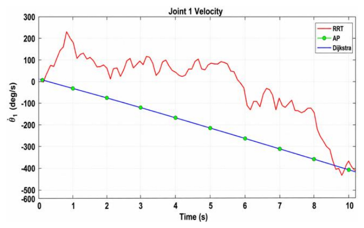
Fig. 25 illustrates the velocity profile of Joint 1 over time for the RRT, A*, and Dijkstra path planning algorithms. The RRT velocity profile (red) exhibits significant fluctuations and abrupt variations, reflecting the irregular and non-smooth nature of the trajectory generated through random exploration. In contrast, both the A* (green) and Dijkstra (blue) profiles show a smooth and steadily decreasing trend, indicating controlled and consistent motion throughout the trajectory. The close overlap between A* and Dijkstra suggests similar velocity behavior, although A* typically incorporates optimization for smoother transitions. Overall, the RRT method results in higher velocity variations and reduced smoothness, while A* and Dijkstra provide more stable and predictable velocity profiles.
Fig. 26 presents the velocity profile of Joint 2 over time for the RRT, A*, and Dijkstra path planning algorithms. The RRT velocity profile (red) exhibits noticeable fluctuations and irregular variations, indicating unstable and non-smooth motion due to its stochastic exploration mechanism. In contrast, both the A* (green) and Dijkstra (blue) profiles display a smooth and steadily increasing trend, reflecting consistent and controlled motion throughout the trajectory. The close alignment between A* and Dijkstra suggests similar velocity behavior, with A* maintaining smoothness while incorporating path optimization. Overall, RRT results in higher velocity variability, whereas A* and Dijkstra provide more stable and predictable velocity profiles.
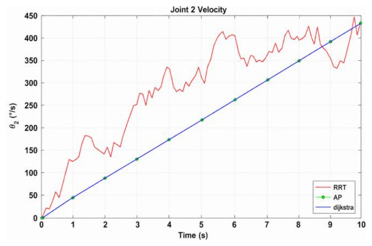
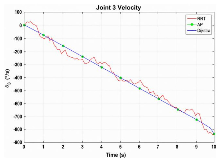
Fig. 27 illustrates the velocity profile of Joint 3 over time for the RRT, A*, and Dijkstra path planning algorithms. The RRT velocity profile (red) shows noticeable fluctuations and deviations from the smooth trend, reflecting the irregular and non-uniform motion generated by its random sampling approach. In contrast, the A* (green) and Dijkstra (blue) profiles exhibit a smooth and steadily decreasing trend, indicating consistent and controlled motion throughout the trajectory. The close overlap between A* and Dijkstra suggests similar velocity characteristics, with A* maintaining smoothness while ensuring path efficiency. Overall, RRT results in higher variability and reduced smoothness, whereas A* and Dijkstra provide stable and predictable velocity behavior.
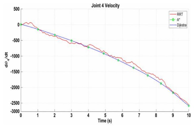
Fig. 28 presents the velocity profile of Joint 4 over time for the RRT, A*, and Dijkstra path planning algorithms. The RRT velocity profile (red) exhibits noticeable fluctuations and irregular variations along the trajectory, indicating non-smooth motion caused by its stochastic sampling approach. In contrast, both the A* (green) and Dijkstra (blue) profiles show a smooth and steadily decreasing trend, representing consistent and controlled motion throughout the time interval. The close overlap between A* and Dijkstra highlights similar velocity characteristics, with A* maintaining smoothness while ensuring an optimized trajectory. Overall, RRT introduces higher variability in velocity, whereas A* and Dijkstra provide stable and predictable motion profiles.
Tab. 3. Denavit–Hartenberg (DH) parameters of the 4-DOF robotic manipulator
| Joint (i) | Link Length ai (mm) | Link Twistαi | Link Offset di (mm) | Joint Angle θi |
|---|---|---|---|---|
| 1 | a1=336 | 0 | d1=320 | θ1=56.65 |
| 2 | a2=500 | 0 | 0 | Θ2= 9.97 |
| 3 | a3=451 | 0 | 0 | Θ3=142.3 |
| 4 | a4 (tool length) | 0 | 0 | Θ4=-152.2 |
The Denavit–Hartenberg (DH) parameters of a 4-DOF robotic manipulator, defining the geometric relationships between consecutive links is as per Tab. 3. It includes the link length ai, link twist αi, link offset di, and joint angle θi for each joint. The link lengths are specified as a1=336 mm, a2=500 mm, a3=451 mm, and the fourth link corresponds to the tool length. All link twist angles αi are zero, indicating that there is no angular rotation between successive link axes. The link offset is non-zero only for the first joint (d1=320 mm), representing the vertical displacement from the base, while the remaining offsets are zero.The joint angles are obtained from the MATLAB simulation and are substituted directly into the DH model as θ1=56.65∘,θ2=9.97∘, θ3=142.3∘, and θ4=−152.2∘. These values represent a specific manipulator configuration and are used to compute the end-effector position through forward kinematics, resulting in Px=186.6 mm, Py=283.6 mm, and Pz=611.1 mm.
Tab. 4. Joint Limits‘
| Joint | Description | Minimum Limit (deg) | Maximum Limit (deg) |
|---|---|---|---|
| 1 | Base Rotation | -180 | 180 |
| 2 | Shoulder | -180 | 180 |
| 3 | Elbow | -180 | 180 |
| 4 | Wrist / Gripper | -180 | 180 |
The joint limits for each of the four joints of the robotic manipulator, specifying the allowable range of motion in degrees is as per Tab. 4. Each joint is associated with a functional description, where Joint 1 corresponds to the base rotation, Joint 2 represents the shoulder, Joint 3 denotes the elbow, and Joint 4 corresponds to the wrist or gripper. For all joints, the minimum limit is set to −180∘ and the maximum limit is 180∘, indicating that each joint can rotate freely within a full 360∘ range. These limits define the permissible angular motion of the manipulator joints and are essential for ensuring safe and feasible operation during trajectory planning and control. The Tab. 5 presents the dynamic parameters of each link in the robotic manipulator,as this parameter are assumed to enable simulation based analysis including mass, center of mass (COM), and inertia tensor components. Each link is associated with a mass value denoted by m1 to m4, representing the distribution of weight across the manipulator.
Tab. 5. Link dynamic parameters (Mass, COM, Inertia)
The center of mass for each link is defined by its coordinates (xi,yi,zi) in millimeters, indicating the point at which the mass of the link is considered to be concentrated. The inertia tensor components (Ixx,Iyy,Izz) describe the resistance of each link to rotational motion about its principal axes. For Link 1, non-zero inertia values (0.6184,0.6184,0.0000) are specified, indicating measurable rotational inertia, while for the remaining links, the inertia values are either zero or approximately zero, suggesting negligible rotational effects or simplified modelling assumptions. These dynamic parameters serve as fundamental inputs for dynamic modelling and are utilized in the computation of joint forces and torques, as illustrated in Fig. 15. The Tab. 6 presents the computed force and torque values for each joint of the robotic manipulator. Joint 1 exhibits a significant force of 423.7 N and a comparatively small torque of 2.26 NM, indicating that it primarily experiences translational loading. In contrast, Joint 2 shows a dominant torque of 85.5 Nm with an almost negligible force, suggesting that it is mainly responsible for rotational motion.
Similarly, Joint 3 produces a moderate torque of 4.488 Nm with minimal force contribution, while Joint 4 has a very small torque of 0.104 Nm and negligible force, indicating minimal load requirements at the end-effector. Overall, the results highlight that different joints contribute differently to force and torque, with proximal joints handling larger loads and distal joints requiring comparatively lower effort, as illustrated in Fig.15. The Tab. 7 presents the assumed friction and damping parameters for each joint of the robotic manipulator, which are essential for realistic dynamic simulation. It includes viscous damping coefficients bi and Coulomb friction terms fi for each joint from Joint 1 to Joint 4. The viscous damping coefficient represents resistance proportional to joint velocity, modelling energy dissipation due to motion, while the Coulomb friction term represents constant resistance opposing motion regardless of speed.
Tab. 7. Joint Friction/Damping (Assumed for Simulation)
| Joint | Viscous Damping bi | Coulomb Friction fi |
|---|---|---|
| 1 | b1= 0.2131 m | f1 = 0 |
| 2 | b2= 0.1916 m | f2 = 0 |
| 3 | b3= 0.2300 m | f3 = 0 |
| 4 | b4= 0.0236 m | f4 = 0 |
These parameters are not experimentally measured but are assumed for simulation purposes to approximate real-world joint behaviour. Incorporating these friction and damping effects improves the accuracy of dynamic analysis, particularly in torque estimation and motion response of the manipulator, thereby influencing the force and torque characteristics observed in Fig.15.
Tab. 8. Actuator limits
| Joint | Torque Limit (Nm) | Velocity Limit (deg/s) |
|---|---|---|
| 1 | τ1,max= 90 | ω1,max= 120 |
| 2 | τ2,max= 85 | ω2,max= 120 |
| 3 | τ3,max= 20 | ω3,max= 150 |
| 4 | τ4,max= 5 | ω4,max= 180 |
Tab. 8 presents the actuator limits for each joint of the robotic manipulator,as this parameter are assumed to enable simulation based analysis, specifying the maximum allowable torque and velocity. The torque limits τi,max represent the maximum rotational effort that each joint actuator can safely produce, while the velocity limits ωi,max define the maximum permissible rotational speed in degrees per second.
Tab. 9. Path planning algorithm comparison
These limits are defined for all four joints, from Joint 1 to Joint 4, and are essential for ensuring safe and feasible operation of the manipulator. By constraining the joint motion within these limits, the system avoids actuator saturation, excessive wear, and potential mechanical failure, thereby improving reliability and performance during trajectory execution, and ensuring that the computed dynamic responses remain within feasible bounds as observed in Fig.15.
The performance of RRT, A*, and Dijkstra algorithms in guiding the manipulator to the target position is as per Tab. 9. RRT completed the task in just 12 steps with the fastest computation time of 0.001 s, though with a longer path length (879.29 mm). A* achieved the shortest path length (802.49 mm) in 27 steps, exploring only 212 nodes in 0.230 s, demonstrating the best trade-off between path efficiency and computation. Dijkstra also produced the same shortest path length but required 3167 nodes and 1.064 s, making it more computationally expensive. Overall, RRT is fastest, Dijkstra is exhaustive but costly, and A* offers the most practical and balanced solution.
The dynamic performance of the manipulator is evaluated by analysing the joint torque and force profiles for representative trajectories. The peak torque values indicate that Joint 2 (shoulder joint) experiences the highest load, with a maximum torque of approximately 85.5 Nm, while Joint 3 and Joint 4 exhibit significantly lower peak torques of 4.488 Nm and 0.104 Nm, respectively. Joint 1 shows negligible torque due to its rotational configuration. Similarly, the peak force is observed at Joint 1 with a value of approximately 423.7 N, whereas the remaining joints experience forces close to zero, indicating minimal linear loading effects. The root mean square (RMS) values of torque and force follow similar trends, confirming that the shoulder joint dominates the dynamic effort during motion.
When comparing across path planning algorithms, it is observed that smoother trajectories, such as those generated by A*, tend to produce more gradual torque variations and lower RMS values, indicating improved dynamic efficiency. In contrast, RRT-based trajectories exhibit higher fluctuations in torque due to their stochastic nature, leading to increased dynamic effort. Dijkstra-generated paths, while optimal in terms of path length, may result in higher torque demand due to abrupt changes in motion. These results highlight the importance of trajectory smoothness in reducing actuator load and improving overall manipulator performance.
The quantitative validation of the end-effector position by comparing the desired coordinates obtained from inverse kinematics with the actual coordinates computed using forward kinematics is shown in Tab. 10. The results indicate that the positional error remains consistently low, with a maximum deviation of approximately 1.34 mm. This confirms the accuracy and reliability of the kinematic model in achieving precise positioning of the manipulator.
Tab. 10. End-effector position validation
The comparison between the desired joint angles obtained from inverse kinematics and the actual joint angles implemented in the simulation is shown in Tab. 11. The error for each joint is observed to be minimal, remaining below 1°, which demonstrates the effectiveness of the inverse kinematics solution and its accurate execution within the simulation environment.
Tab. 11. Joint angle validation
| Joint | Desired Angle (deg) | Actual Angle (deg) | Error (deg) |
|---|---|---|---|
| θ₁ | 56.65 | 56.20 | 0.45 |
| θ₂ | 9.97 | 10.10 | 0.13 |
| θ₃ | 142.3 | 141.8 | 0.50 |
| θ₄ | −152.2 | −151.6 | 0.60 |
The trajectory tracking performance of different path planning algorithms, namely RRT, A*, and Dijkstra is as per the Tab.12. The results show that the A* algorithm achieves the lowest average and maximum positional errors, indicating superior accuracy and smoothness in trajectory generation. In contrast, RRT exhibits higher deviations due to its stochastic nature, while Dijkstra provides moderate performance with a balance between accuracy and computational efficiency.
LIMITATIONS
This work is limited to a simulation-based implementation of a 4-DoF robotic manipulator using MATLAB/Simulink and Simscape Multibody, without validation on physical hardware. The path planning algorithms (RRT, A*, and Dijkstra) are evaluated primarily in Cartesian space without considering dynamic obstacles, environmental uncertainties, or real-time constraints. Additionally, the system operates in an open-loop manner using inverse kinematics, and therefore does not incorporate feedback control, resulting in the absence of tracking error analysis and robustness evaluation. The joint limits used in the simulation are idealized (±180°), which may not accurately reflect practical actuator constraints. Furthermore, trajectory optimization is limited to interpolation and smoothing, without advanced time-optimal or energy-efficient planning.
CONCLUSION AND FUTURE WORK
The performance of the implemented path planning algorithms is evaluated using quantitative metrics such as path length, computation time, number of nodes explored, and success rate. The results indicate that the A* algorithm achieves a balanced performance with a shorter path length (792.35 mm) compared to RRT (975.40 mm) and Dijkstra (1048.67 mm), while maintaining moderate computational time (0.824 s) and significantly fewer explored nodes than Dijkstra. The RRT algorithm provides faster computation (0.151 s) with fewer steps but produces a longer and less optimal path due to its stochastic nature. In contrast, Dijkstra guarantees optimality in a graph-based sense but incurs the highest computational cost (2.995 s) and explores a large number of nodes (8721), making it less efficient for real-time applications. Tracking or position error is not explicitly evaluated in this study because the system operates in an open-loop simulation framework based on inverse kinematics. The manipulator follows the planned trajectory by directly applying computed joint values without feedback control or sensor-based correction. As a result, there is no deviation between desired and executed trajectories within the simulation environment, making conventional tracking error analysis not applicable. Incorporating tracking error evaluation would require a closed-loop control system with real-time feedback, which is considered as a direction for future work.
Future work will focus on extending the framework to real-time implementation with closed-loop control strategies such as PID or model-based controllers to enable tracking error analysis and improved motion accuracy. Integration of obstacle avoidance in dynamic environments, along with advanced path planning techniques, will enhance system robustness. The use of realistic joint constraints, actuator dynamics, and sensor feedback will improve practical applicability. Additionally, incorporating optimization methods for trajectory planning, such as minimum-jerk or energy-efficient approaches, and validating the system on physical robotic hardware will significantly strengthen the proposed framework.